
“
Problem-oriented, starting from scratch, quickly getting hands-on, efficiently learning, and mastering Matlab programming.
”
The previous posts in the Matlab beginner tutorial | 008 Two-dimensional Plotting: A Comprehensive Guide to the Use of plot and Matlab Beginner Tutorial | 010 Introduction to the Universal Formula for Matlab Plotting introduced the basic knowledge of Matlab plotting and some parameter settings. Mastering this knowledge allows you to create graphs for your papers using Matlab.
Today we will explore some advanced Matlab plotting techniques. Sometimes, when we want to create a certain effect in Matlab, we encounter significant challenges. For example, coordinate systems are one of them, as well as color filling, bezier curves, tangents to curves, and color matching issues, etc. Sometimes, due to the lack of ready-made functions, we need to go through advanced skills such as calculating and programming to achieve the desired effect when plotting.
Fashionable Tech Style vs Classic Textbook Style
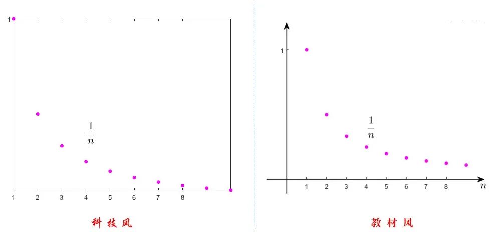
First, let’s talk about coordinate systems. The coordinate system provided by Matlab is a framed, arrowless system where the intersection of the axes is generally not at the origin. Its advantage is that when presenting scatter plots, contour lines, images, etc., it is not disturbed by the coordinate system, giving it a fashionable tech style.
However, in mathematical textbooks and exams, we prefer to use the classic coordinate system: where the axes intersect at the origin and have arrows. This type of coordinate system is particularly intuitive and convenient for illustrating the zero points of function curves, the positivity and negativity of function values, and the relationship between surfaces and planes.
Unfortunately, the developers of Matlab did not intend to provide such a classic coordinate system, or they believed that it could be easily created using existing functions. Indeed, Matlab experts have written functions to draw such classic coordinate systems themselves.
For example, <span>shift_axis_to_origin.m</span> is used to draw classic coordinate systems. It shifts the axes to the origin through programming and adds arrows to the axes. After testing, I found that in most cases, it can produce satisfactory graphs, but it does not work well with the <span>axis equal</span> command, so it is best to avoid using that command.
When calling <span>shift_axis_to_origin.m</span>, save it in the current folder and call it with the following statement:
shift_axis_to_origin(gca);
bezier Curves
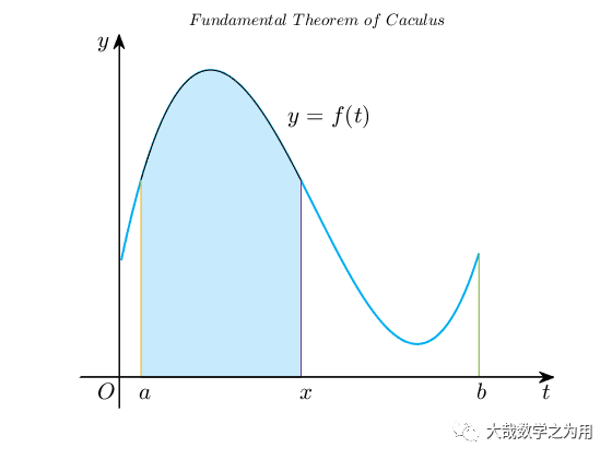
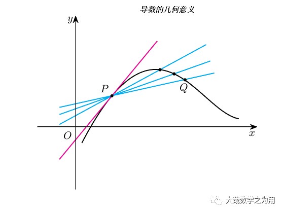
The two images below, “Geometric Meaning of Derivatives” and “Geometric Meaning of Definite Integrals”, contain curves that are drawn using bezier curves. Matlab does not provide a function to draw bezier curves either. Matlab experts have created their own functions for drawing bezier curves through programming. To draw any curve using the bezier function, one needs to try continuously changing the parameter values to achieve the desired curve effect, which is a challenging and tedious task.
Color Filling
The color filling function is <span>fill</span>, and its usage format is:
fill(X,Y,colorspec)
<span>fill</span> treats the pair (X,Y) as a “polygon” and fills it with color <span>colorspec</span>. If the given data does not form a closed shape, it automatically connects the endpoint to the starting point to close it. The <span>colorspec</span> can be default colors like <span>r,g,b,c,k</span> representing “red, green, blue, cyan, black” etc.; or it can be custom colors specified by <span>rgb</span> values, where the values of <span>r,g,b</span> are numbers in the range.
To get the <span>RGB</span> values of a color block on the screen: when using WeChat, press <span>Alt+A</span>, or when using QQ, press <span>Ctrl+Alt+A</span>, then move the mouse over the color block to view its RGB values. This is a three-element array, each number being an integer between 0 and 255.
You can enter in the Matlab command window:
[199 234 252]/255
This will calculate its <span>rgb</span> value to be: [0.78 0.92 0.99]. Thus,
fill(X,Y,[0.78 0.92 0.99])
can be used to fill with this custom color.

Color Matching
The colors pre-defined in Matlab tend to be too dark and heavy. Using these colors to fill shapes can make them feel overwhelming, glaring, or oppressive. Therefore, we need to stock up on some more beautiful color <span>rgb</span> values for use.
Tangents
It seems that Matlab does not have a function to draw tangents. If the curve does not have an expression, an approximate method can be used: for example, to draw the tangent at a point on a bezier curve, one can take the coordinates of points nearby (hovering over the point can display the coordinates) to use the slope of the secant as an approximation for the slope of the tangent.
Mathematical Formula Labels
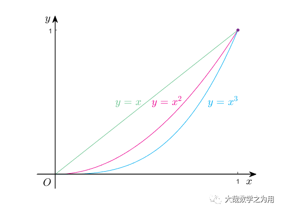
The default font for mathematical formulas in Matlab is unattractive, but it provides a function to call the <span>LaTeX</span> package, allowing us to create beautiful mathematical formula labels.
You can refer to the format below:
text('Interpreter','latex','String','$$y=x^2$$','Position',[1.02,1],'FontSize',16);
title('$$Area\ under\ y = x^2\ on\ [0,1]$$','Interpreter','latex','FontSize',17)
<span>text</span> is used for textual annotations for graphs and axis names. <span>interpreter,latex</span> indicates that the following formula part is to be interpreted using latex. The formula is enclosed in double $ symbols, which is the display method for block formulas.<span>position,[1.02,1]</span> indicates that the label’s position is at coordinates [1.02,1].<span>FontSize,16</span> indicates that the font size of the formula is <span>16pt</span>.
<span>title</span> is used to label the name of the graph, displayed at the top of the graph frame, centered. Its format is slightly different from that of <span>text</span>.

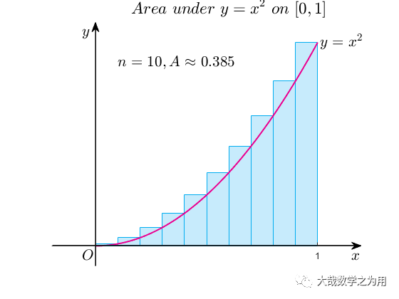
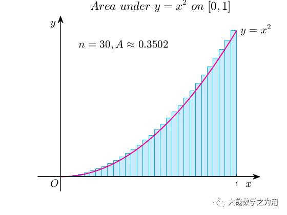
Combining Two Plotting Functions
In the following example, “Definition of Definite Integrals”, we use the area of vertical rectangles to approximate the area of the curved trapezoid. We simultaneously used the <span>fplot</span> function and the <span>bar</span> function, using the former to draw curves and the latter to draw vertical rectangles.
It is necessary to set the property parameters of the <span>bar</span> function to change its width, edge color, and fill color:
bar(x,y,1,'facecolor',[0.78 0.92 0.99],'edgecolor',[0 0.68 0.94]);

Today’s content ends here. Friends who prefer classic coordinate systems will surely find inspiration from these examples.
The code for the examples mentioned in the article has been packaged and uploaded to Baidu Cloud. Friends in need can long press the QR code below to obtain:
Long press to recognize the QR code below, reply to the public account:caxis to receive!

Long press to recognize the QR code to reply:003, receive video and e-book
Long press the QR code above, reply:003, to receive 2.5G of Matlab videos + beginner to advanced e-books!
[1] Charles F. Van Loan, K. V. Daisy Fan, Insight Through Computing.
[2] Zhang Zhiyong, Mastering MATLAB R2011A.


Welcome to “like”, ‘“see” and leave a message! Your support is our motivation to continue!