MATLAB Signal Simulation | Understanding Frequency Resolution of Fourier Transform

1. What is Zero Padding?

Simply put, zero padding is the process of adding several zeros to the end of a time-domain or spatial-domain signal before transformation to increase the data length. As shown in Figure 1, this is a real sine wave signal composed of two frequency components at 1.00 MHz and 1.05 MHz.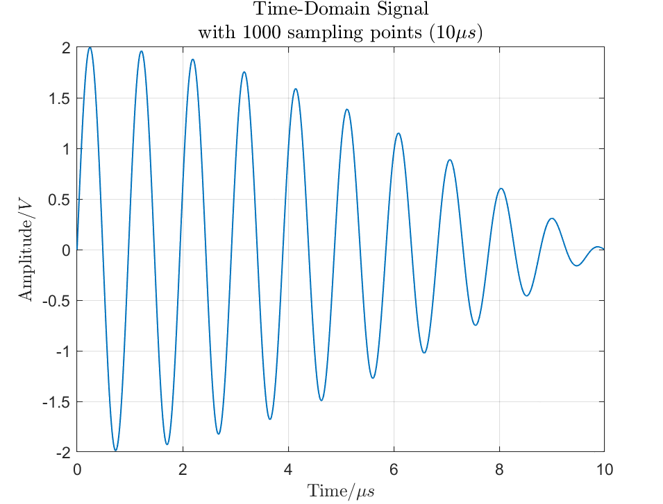

(a) Original Signal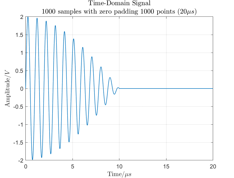

(b) Zero-Padded Signal

Figure 1: Illustration of Zero Padding in Time Domain

In the signal shown in Figure 1(a), the signal length is 1000 samples, and with a sampling frequency of 100 MHz, the actual length of the signal is 10 microseconds.

By adding 1000 zeros at the end, the data length increases to 2000 points, resulting in the waveform shown in Figure 1(b).

This process is what is commonly referred to as zero padding.

2. Why is Zero Padding Necessary?

The most direct reason is that if the number of data points in the time-domain waveform is a power of 2, the FFT computation will be most efficient. Hardware (FPGAs) computing FFT uses this padding approach. So, does zero padding affect the frequency resolution of the computed output?

3. About FFT Frequency Resolution

This involves two different meanings of the resolution issue.

One is called waveform frequency resolution, or visual frequency resolution.

The other is referred to as FFT resolution. Although this classification and naming may not necessarily be professional terminology, it helps in understanding the concept of “frequency resolution”.

In the absence of zero padding, these two concepts are usually easy to confuse because they are equivalent.

Waveform frequency resolution refers to the minimum spacing between two distinguishable frequencies; while FFT resolution refers to the number of data points in the spectrum, which is directly related to the number of points used in the FFT.

Therefore, waveform frequency resolution can be defined as:

where T is the time duration of the signal.

Similarly, FFT resolution can be defined as:

where fs is the sampling frequency and NFFT is the number of FFT points. It represents the spacing of frequency values on the FFT frequency axis.

It is important to note that one may have good FFT resolution but still may not be able to easily separate two frequency components.

Likewise, one may have high waveform resolution, but the peaks of the waveform energy may spread across the entire spectrum due to the phenomenon of frequency leakage in FFT.

We know that the Discrete Fourier Transform (DFT) or Fast Fourier Transform (FFT) computes based on an infinite sequence formed by zero padding on either side of the waveform. This is why each frequency bin in the FFT has a distinct functional shape.

Waveform frequency resolution is equivalent to the space between nulls of a function.

4. Example Analysis

Below, we take a periodic signal with two frequency components of 1 MHz and 1.05 MHz as an example to illustrate the relationship between zero padding and resolution. The simulation signal can be written as:

It can be seen that the frequency spacing between the two signals is 0.05 MHz.

That is, we can see the peaks of the two frequency points on our frequency spectrum analysis curve. If the amplitudes of the two sine waves are 1 volt, then we expect the power at the frequencies of 1.00 MHz and 1.05 MHz to be 10 dBm.

Let’s analyze the following situations:

1. FFT Points = Time Domain Samples

Specifically, for equation (3), we sample in the time domain with 1000 points and perform an FFT with the same number of points.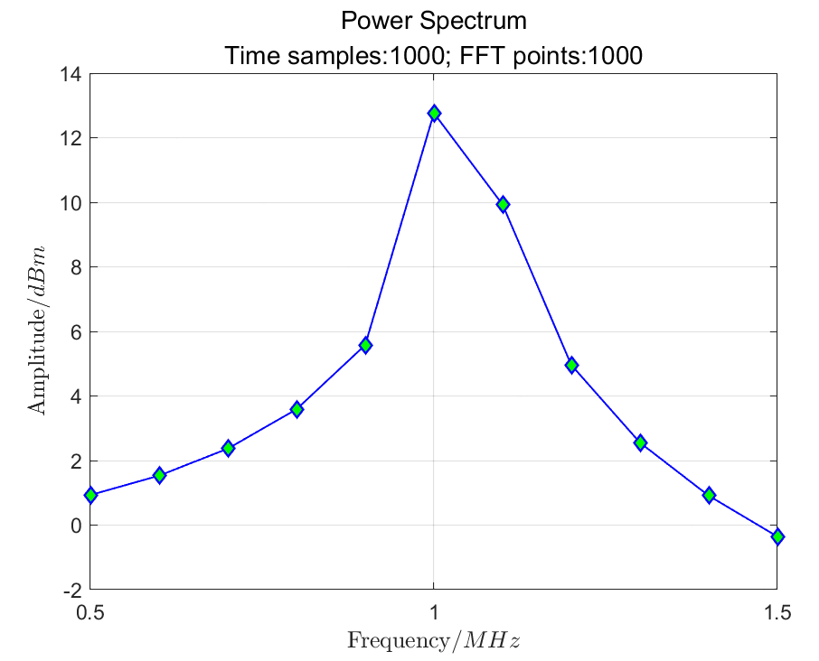

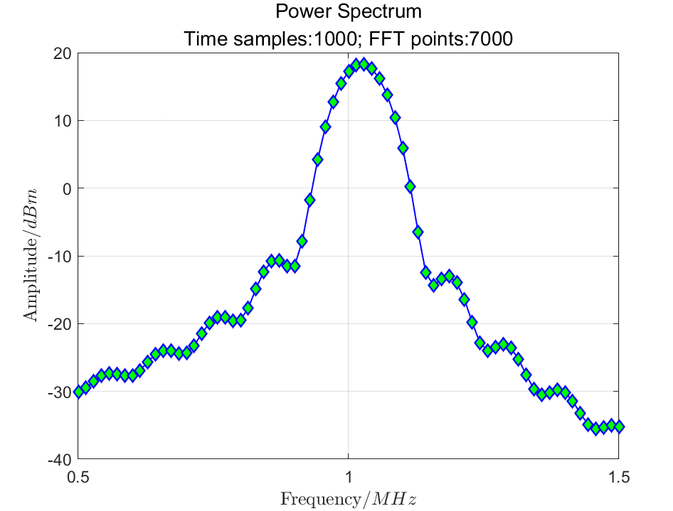
Figure 2: Power Spectrum of Original Signal (1000-Point FFT)

In Figure 2, we do not see the expected two pulses; only one pulse point appears with an amplitude of about 11.4 dBm. Clearly, this graph does not represent the correct frequency spectrum we want.

The reason is simple: there is not enough resolution to see the two peaks.

2. FFT Points > Time Domain Samples

Specifically, for equation (3), we sample in the time domain with 1000 points and perform an FFT with 7000 points.

We naturally think of using zero padding to increase the number of FFT points so that more points can be added to the frequency axis. Using 7000 points for the FFT requires adding 6000 zeros to the end of the original 1000-point signal, resulting in a time length of 60 microseconds. The original signal becomes as shown in Figure 3(a), and its FFT result is shown in Figure 3(b).

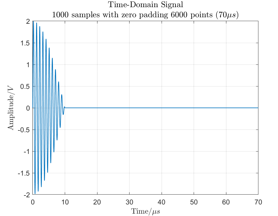(a) Time Domain Signal with 1000 Points, Adding 6000 Zeros

(b) Power Spectrum after 7000 Points FFT of Zero-Padded Signal

In this figure, we also do not see the expected result.

Upon closer observation, this graph tells us something: by increasing the number of FFT points, the definition of the function in the equation for waveform frequency resolution becomes clearer. It can be seen that the spacing between waveform nulls is approximately 0.1 MHz.

Since the frequency interval of the two sine waves is 0.05 MHz, no matter how many FFT points we add through zero padding, we cannot resolve the two sine wave issues.

Now, let’s look at what frequency resolution tells us. Although the FFT resolution is approximately 14 kHz (sufficient frequency resolution), the waveform frequency resolution is only 100 kHz.

The frequency spacing of the two signals is 50 kHz, so we are limited by the waveform frequency resolution.

3. Increasing Time Domain Sampling Points, Performing FFT with Same Number of Points

Specifically, for equation (3), we sample in the time domain with 7000 points and perform a 7000-point FFT.

To reasonably solve this frequency spectrum problem, we need to increase the length (number of points) of the time-domain data used for the FFT.

Thus, we directly collect 7000 points of the waveform as the input signal, replacing the zero padding method (7000 points). The time-domain signal and corresponding power spectrum are shown in Figures 4a and 4b, respectively.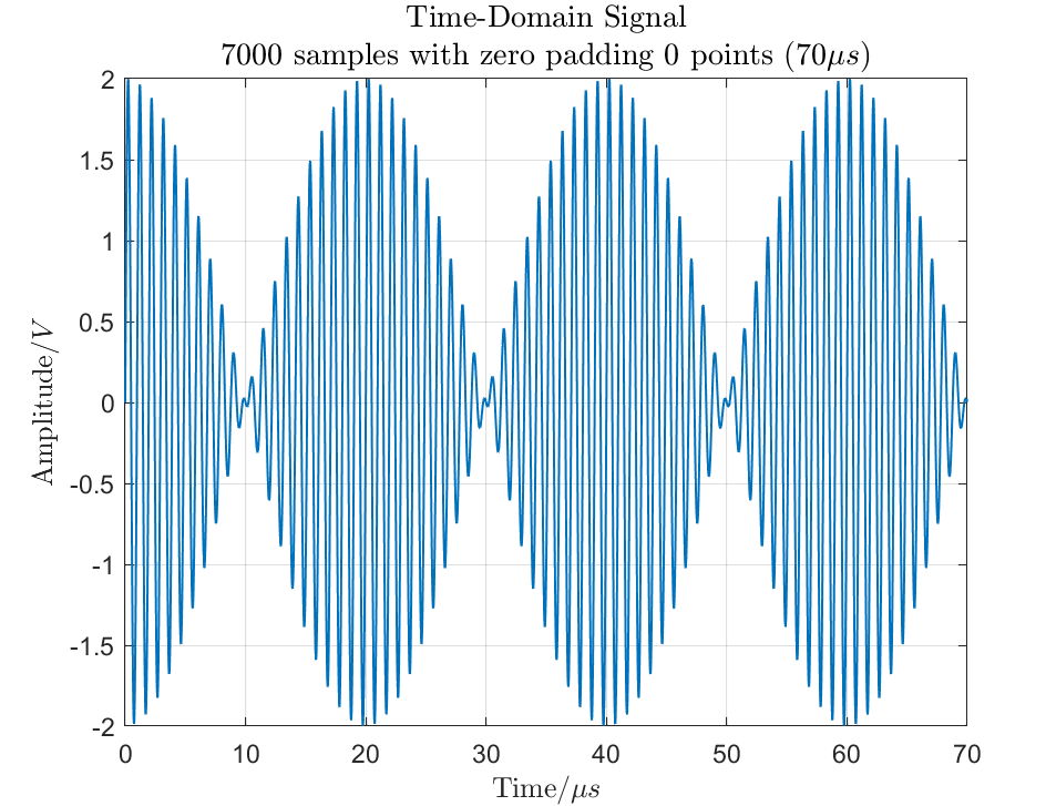

(a) Time Domain Signal with 7000 Points Sampled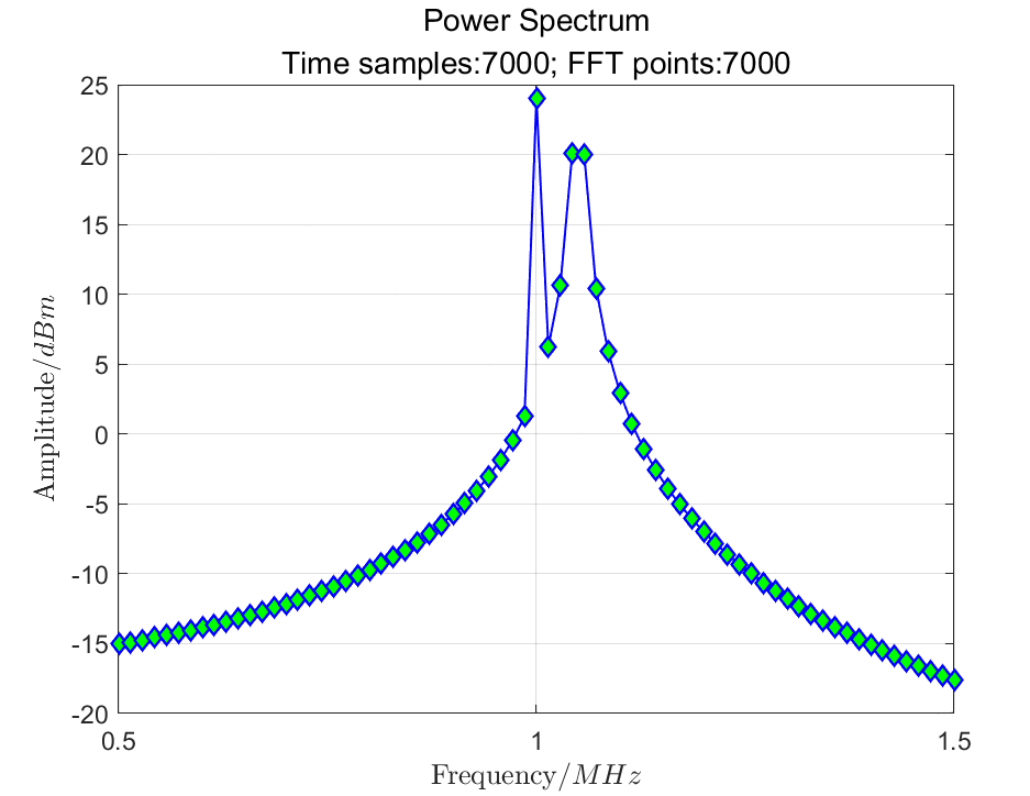

(b) Power Spectrum Calculated from 7000 Point FFT

Figure 4: Signal Sampled at 7000 Points and Its Power Spectrum

By extending the time-domain data, the current waveform frequency resolution is also approximately 14 kHz. From the frequency spectrum, we still do not see the two sine waves. The 1 MHz signal is clearly represented with the correct power of 10 dBm, while the 1.05 MHz signal is broadened and not distributed at the expected 10 dBm power.

Why is this?

The reason is that there is no distribution of FFT points at 1.05 MHz, as the energy is dispersed across multiple FFT points.

In the example given, the sampling frequency is 100 MHz, and the number of FFT points is 7000.

In the frequency spectrum, the spacing between points is 14.28 kHz. The 1 MHz frequency coincides exactly with the integer multiple of the frequency spacing, while 1.05 MHz does not. The nearest integer multiple frequencies to 1.05 MHz are 1.043 MHz and 1.057 MHz, hence the energy is dispersed across these two FFT bins.

4. Increasing Time Domain Sampling Points, Using Zero Padding to Increase Sample Points for FFT

This involves sampling with 7000 points in the time domain and then adding 1000 zeros to perform an 8000-point FFT.

To solve this issue, we can reasonably choose the number of FFT points so that these two points can become independent points on the frequency axis.

Since we do not need better waveform frequency resolution, we only need to use the zero padding method on the time-domain data to adjust the frequency spacing of the FFT data points.

By adding 1000 zeros to the time-domain signal, the frequency spacing becomes 0.05 MHz, thus satisfying that both frequencies are integer multiples of this spacing. The resulting power spectrum is shown in Figure 5. It can be seen that the two frequency issues are resolved, and the power is distributed at the expected 10 dBm.

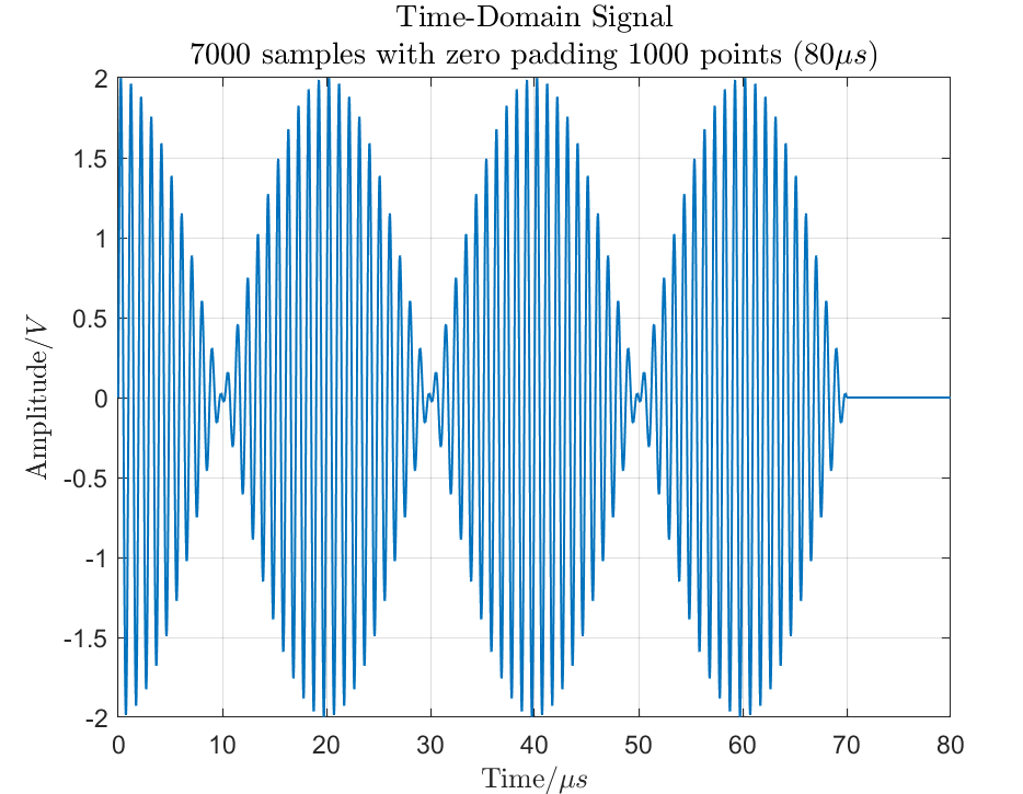(a) Time Domain Signal Sampled at 7000 Points, Zero-Padded with 1000 Points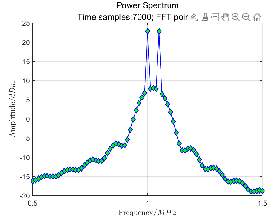(b) Power Spectrum Calculated from 8000 Points FFT

Figure 5: Power Spectrum of Zero-Padded Signal to 8000 Points

To further observe the phenomenon of excessive zero padding, by adding more zero values in the time domain (e.g., 100000 points) to achieve multi-point FFT, we can ensure the correct shape of the FFT units (sinc interpolation), as shown in Figure 6.

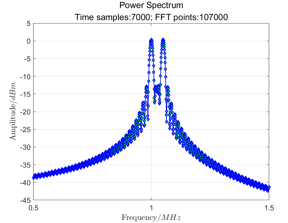
Figure 6: Power Spectrum of Zero-Padded Signal to 107000 Points

All results above were simulated and verified using MATLAB.

The complete code is as follows for reference.

%=========================================================================
%  Demo:  FFT ZeroPadding and Frequency Resolution
%-----------------------------------------
%  Parameter description:
%     dt:   Sampling time interval;
%     T:    Length of signal x (s);
%     N:    Number of sampling points of time-domain signal x (integer):    N = T/dt+1;
%     fs:   Sampling frequency (Hz):               fs = 1/dt;
%     fn:   Nyquist frequency:                fn = fs/2;
%     nfft: FFT points (can be set by user, default is the number of time-domain samples);
%     For real signals, the effective number of points is nfft/2+1, which can be bounded by fn.
%     Data beyond fn is redundant (equivalent to negative half-axis frequency) and can skip fftshift operation.
%
%     df:   Frequency (spacing) precision:              df = fs/nfft;
%     
%  Changing nfft may reduce df and affect the spectral fineness. If the original signal is long enough, the impact is not significant.
%  Because MATLAB matches n to nfft by zero padding or truncating, by default: nfft is consistent with n.
%          
%  Copyright (c) 2006-2024 Zhenming Peng
%  IDIPLAB,
%  School of Information and communication engineering,
%  University of Electronic Science and Technology of China
%
% Revised: 2024.2.15
%=========================================================================
clc; clear; close all;

%-----------------------------------------
% Parameter settings
T  = 10e-006;   % Length of signal(L=10us)
N0 = 1000;      % The number of sampling points of signal

dt = T/N0;      % Time spacing or sampling time
fs = 1/dt;      % Sampling frequency
R  = 50;        % System impedance (ohms)

%-----------------------------------------
% Discretize the original signal and plot the time-domain curve
%-----------------------------------------
% Calculate the corresponding x for each time point t, N is the actual number of sampling points (can be adjusted ✓) 
N = N0 + 6000;     % The number of sampling points 
t = dt*(0:N-1);    % Time vector
x = sin(2*pi*1000000*t) + sin(2*pi*1050000*t); % Signal vector

% Plot the original signal x
plot(t*1e+006,x,'LineWidth',1.0)   % Unit: us
nstr  = num2str(N);
tnstr = num2str(N/100);
title(['Time-Domain Signal',newline,...
    'with ',nstr,' sampling points (',tnstr,'$\\mu s$)',...
    'FontSize',12,'Interpreter','Latex');
xlabel('Time/$\mu s$','Interpreter','Latex');
ylabel('Amplitude/$V$','Interpreter','Latex')
grid on
set(gcf,'Color','w')

% Zero-padding in time domain (can be adjusted ✓) 
Np = N + 0;         % Zero-padding points 
tp = dt*(0:Np-1);
xp = zeros(1,Np);   % All zeros in xp
xp(1:N) = x;        % Zero-padding

tp = tp*1e+006;     % Unit conversion: s -> us
figure,
tnstr =  num2str(Np/100);
plot(tp,xp,'LineWidth',1.0)
title(['Time-Domain Signal',newline,num2str(N),...
    ' samples with zero padding ', num2str(Np-N),...
    ' points (',tnstr,'$\\mu s)$',...
    'FontSize',12,'Interpreter','Latex')
xlabel('Time/$\mu s$','Interpreter','Latex');
ylabel('Amplitude/$V$','Interpreter','Latex')
grid on
set(gcf,'Color','w')
%-----------------------------------------

nfft = Np;                          % FFT points
%nfft = 2^nextpow2(nfft); % Next power of 2 from length of x
%-----------------------------------------

% FFT
%-----------------------------------------
Y = fft(x,nfft);                    % Zero-padding or truncation according to x
%Y = fftshift(Y);                   % Centering the spectrum
Fy = abs(Y)./ nfft;                 % Normalized amplitude spectrum
Py = 10.*log10(((Fy.^2)/R)*1000)*2; % Power spectrum (dBm)
%-----------------------------------------

% Frequency axis coordinates (scale) values
%-----------------------------------------
df = fs/nfft;                      % Frequency spacing (precision)
f = df*(0:floor(nfft/2)-1)/1e+006; % Only take real frequency, unit conversion (Hz -> MHz)
%-----------------------------------------

% Power spectrum calculation and plotting
%-----------------------------------------
figure,
plot(f,Py(1:floor(nfft/2)),'-bd','MarkerFaceColor',...
    'g','LineWidth',1.0);          % Real frequency (half cycle)
title(['Power Spectrum',newline,'Time samples:',num2str(N),...
    '; ','FFT points:',num2str(nfft)],'FontSize',12);
xlabel('Frequency/$MHz$');
ylabel('Amplitude/$dBm$');
ax = gca; grid on
ax.YLabel.Interpreter = 'Latex';
ax.XLabel.Interpreter = 'Latex';
xlim([0.50,1.50]);         % Only display the local data
set(gcf,'Color','w')

To complete the above simulation verification, the parameters that need to be modified and adjusted are N0 and N, mainly in two places in the program code:

1) N variable: number of time-domain samples, code block as follows:

% Calculate the corresponding x for each time point t, N is the actual number of sampling points (can be adjusted ✓) 
N = N0 + 6000;     % The number of sampling points 

Where N0 = 1000 is the base sample, and 6000 is the additional sample points, making the total time-domain sample 7000 samples.

2) Np variable: represents the total number of points, code block as follows:

Np = N + 1000;     % Zero-padding points 

Where N is the number of time-domain samples, and 1000 is the number of zero padding points.

Finally, two additional notes:

1) Unit Conversion

To obtain a reasonable labeling of the amplitude of the time-domain signal corresponding to voltage (V), it needs to be converted in accordance with the square absolute value of the signal power and voltage.

At the same time, the power labeling of the frequency-domain signal also needs to consider the system impedance because power is defined as: P = V^2/R.

Typically, electrical engineers express power in dBm, so the power spectrum in the code is expressed in dBm. The formula for calculating power spectrum energy is as follows:

2) Normalization of Power

In practical applications, the power of the discrete signal’s FFT needs to be normalized to account for the length of the time-domain signal.

References

[1]http://www.bitweenie.com/listings/fft-zero-padding/

[2]https://www.bitweenie.com/listings/power-spectrum-matlab/

[3]https://www.bitweenie.com/listings/fft-frequency-axis/