Today, we will explore common model algorithms and MATLAB code used in mathematical modeling. I hope this article will be helpful! Don’t forget to like and support at the end of the article. Let’s take a look at the table of contents!1、Monte Carlo Algorithm2、Data Fitting3、Data Interpolation4、Graph TheoryShortest Path ProblemDijkstra Algorithm
1
Monte Carlo Algorithm
1、Definition The Monte Carlo algorithm is a numerical computation method based on probability and statistical theories and methods. It relates the problem to be solved with a certain probability model and uses a computer to implement statistical simulation or sampling to obtain an approximate solution to the problem, hence also known as the random sampling method or statistical experimental method. 2、Scope of Application It can effectively solve complex mathematical computation problems such as multiple integral calculations, differential equation solving, integral equation solving, eigenvalue calculations, and solving nonlinear equation systems. 3、Characteristics The Monte Carlo algorithm can be applied in many scenarios, but it seeks approximate solutions. The larger the simulated sample size, the closer it gets to the true value. Increasing the number of samples significantly increases the computational load. For some simple problems, Monte Carlo is a clumsy method, but for many problems, it is often an effective, sometimes even the only feasible method. 4、Example y = x^2, y = 12 – x forms a curved triangle with the X-axis in the first quadrant. Design a random experiment to estimate the area of this shape.(1) Plotting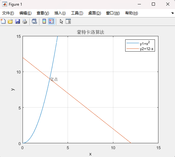 Code
Code
% Plotting
x = 0:0.25:12;
y1 = x.^2;
y2 = 12 - x;
plot(x, y1, x, y2)
xlabel('x');
ylabel('y');
% Generate legend
legend('y1=x^2', 'y2=12-x');
title('Monte Carlo Algorithm');
% Set the range for x and y axes, the range before the brackets is for y-axis, and after is for x-axis
axis([0 15 0 15]);
text(3, 9, 'Intersection');
% Add grid lines
grid on
(2) The idea of the designed random experiment: Generate 10^7 random points uniformly distributed in the rectangular area [0,12]*[0,9], and count the number of random points that fall within the curved triangle. The area of the curved triangle is approximately equal to the area of the rectangle multiplied by the frequency.Code:
% Specific implementation of the Monte Carlo algorithm
% Generate a matrix with 1 row and 10000000 columns, where each number is randomly taken from 0 to 12
x = unifrnd(0, 12, [1, 10000000]);
y = unifrnd(0, 9, [1, 10000000]);
frequency = sum(y<x.^2 && x<=3) + sum(y<12-x && x>=3);
area = 12*9*frequency/10^7;
disp(area);
The estimated value = 49.5026
2
Data Fitting
1、Definition Given a finite number of data points, find an approximate function that may not pass through the known data points but minimizes the total deviation from these points in some sense, thus reflecting the overall trend of the data. 2、Common Methods Generally, the least squares method is used.The implementation of fitting is divided into MATLAB and Excel implementations. The MATLAB implementation uses the polyfit function, which is mainly for polynomial fitting. 3、Example The data is as follows:
   Serial Number   x         y       z
1   426.6279  0.066  2.897867
2   465.325   0.123  1.621569
3   504.0792  0.102  2.429227
4   419.1864  0.057  3.50554
5   464.2019  0.103  1.153921
6   383.0993  0.057  2.297169
7   416.3144  0.049  3.058917
8   464.2762  0.088  1.369858
9   453.0949  0.09   3.028741
10  376.9057  0.049  4.047241
11  409.0494  0.045  4.838143
12  449.4363  0.079  4.120973
13  372.1432  0.041  3.604795
14  389.0911  0.085  2.048922
15  446.7059  0.057  3.372603
16  347.5848  0.03   4.643016
17  379.3764  0.041  4.74171
18  453.6719  0.082  1.841441
19  388.1694  0.051  2.293532
20  444.9446  0.076  3.541803
21  437.4085  0.056  3.984765
22  408.9602  0.078  2.291967
23  393.7606  0.059  2.910391
24  443.1192  0.063  3.080523
25  514.1963  0.153  1.314749
26  377.8119  0.041  3.967584
27  421.5248  0.063  3.005718
28  421.5248  0.063  3.005718
29  421.5248  0.063  3.005718
30  421.5248  0.063  3.005718
31  421.5248  0.063  3.005718
32  421.5248  0.063  3.005718
33  421.5248  0.063  3.005718
34  421.5248  0.063  3.005718
35  421.5248  0.063  3.005718
36  421.5248  0.063  3.005718
37  416.1229  0.111  1.281646
38  369.019   0.04   2.861201
39  362.2008  0.036  3.060995
40  417.1425  0.038  3.69532
(1) Method One: Using MATLAB to write code
% Read table
A = xlsread('E:\table\1.xls', 'Sheet1', 'A1:AN2');
B = A;
[I, J] = size(B); % Data fitting
% x is the first row of the matrix, y is the second row
x = A(1,:);
y = A(2,:);
% polyfit is the fitting function in MATLAB, the first parameter is the x-coordinates of the data
% the second parameter is the y-coordinates of the data, the third parameter is the highest degree of the polynomial
% The return value p contains n+1 polynomial coefficients
p = polyfit(x, y, 2);
disp(p);
% Below is the plotting code
x1 = 300:10:600;
% polyval is the evaluation function in MATLAB, which calculates the function value corresponding to x1
% y1 = polyval(p,x1);
plot(x,y,'*r',x1,y1,'-b');
% plot(x,'DisplayName','x','YDataSource','x');
% figure(gcf);
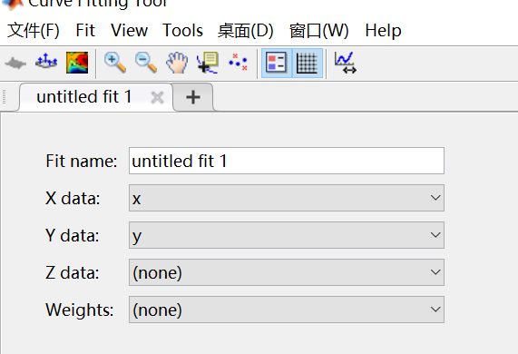
(2) Method Two: Using MATLAB’s graphical fitting toolbox (recommended)Import the data into the workspace and open MATLAB’s graphical fitting toolbox using the cftool command.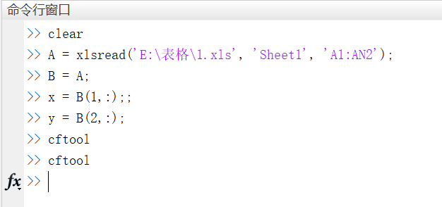 Select x and y variables
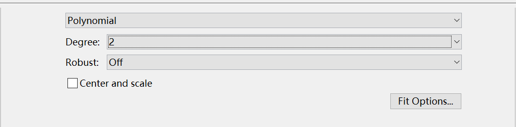
 Select fitting method and highest degree
 Obtain fitting results
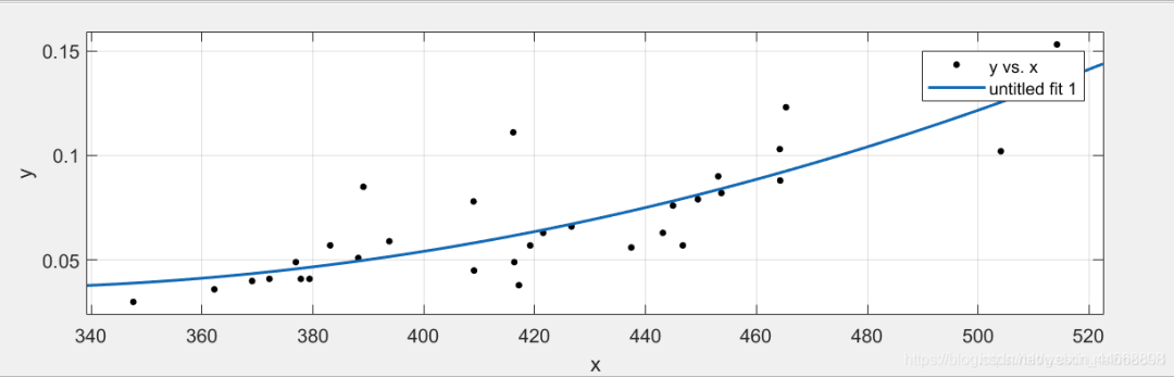 Using the graphical fitting tool is not only simple and quick but also allows for various fitting methods to find the best fitting curve.
3
Data Interpolation
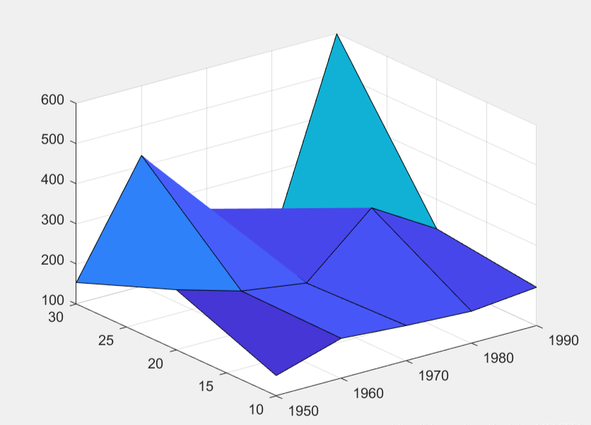
1、Definition Interpolation is the process of filling in continuous functions based on discrete data, ensuring that the continuous curve passes through all given discrete data points. It seeks an approximate function that passes through a finite number of known data points.From the definition, interpolation and fitting have some similarities, but interpolation requires the approximate function to pass through all given discrete data, while fitting does not require this, as long as the approximate function can reflect the trend of data changes well (the meaning of approximation is different). When the measured values are accurate and without error, interpolation is generally used; when the measured values have errors compared to the true values, data fitting is generally used. 2、Function Interpolation is an important method for approximating discrete functions, allowing estimation of the function’s approximate values at other points based on its values at a finite number of points. 3、Example
% years, service, and wage are the original data
years = 1950:10:1990;
service = 10:10:30;
wage = [ 150.697  199.592  187.625  179.323  195.072;
250.287  203.212  179.092  322.767  226.505;
153.706  426.730  249.633  120.281  598.243];
[X, Y] = meshgrid(years, service);
% % 3D curve
% plot3(X, Y, wage)
% 3D surface
% figure
surf(X, Y, wage)
% interp2 is the 2D interpolation function in MATLAB, the first two parameters are known positions, the last two are unknown positions, w is the interpolation result at the unknown position
w = interp2(service, years, wage, 15, 1975);
4
Graph Theory
1、Shortest Path Problem The shortest path problem involves selecting the route with the shortest distance.For example: A truck driver is tasked with delivering a load from point A to point B in the shortest time possible. The road network from A to B is complex, with multiple driving routes available. Which route should the driver choose? Assuming the truck’s speed is constant, this problem is equivalent to finding the shortest path from A to B. (Dijkstra Algorithm)
Dijkstra Algorithm
First, provide an undirected graphUse Dijkstra’s algorithm to find the single-source shortest path starting from A. The steps are as follows:
Code Template:
#include<iostream>
#include<cstdio>
#include<cstdlib>
#include<cmath>
#include<cstring>
#include<algorithm>
#include<vector>
#include<fstream>
using namespace std;
const int maxnum = 100;
const int maxint = 2147483647;
int dist[maxnum];     // Represents the shortest path length from the current point to the source point
int prev[maxnum];     // Records the previous node of the current point
int c[maxnum][maxnum];   // Records the path lengths between two points in the graph
int n, line;             // n represents the number of nodes in the graph, line represents the number of paths
void Dijkstra(int n, int v, int *dist, int *prev, int c[maxnum][maxnum]){
    bool s[maxnum];    // Indicates whether the point has been included in the set S
    for(int i=1; i<=n; ++i)      {
        dist[i] = c[v][i];
        s[i] = 0;     // Initially, all points are unused
        if(dist[i] == maxint)              prev[i] = 0;
        else            prev[i] = v;
    }
    dist[v] = 0;
    s[v] = 1;
    // Sequentially take the point with the smallest dist[] value from the points not included in set S and include it in set S
    // Once S contains all vertices in V, dist records the shortest path lengths from the source point to all other vertices
    for(int i=2; i<=n; ++i)      {
        int tmp = maxint;
        int u = v;  // Find the point j with the smallest dist[j] among the currently unused points
        for(int j=1; j<=n; ++j)
            if((!s[j]) && dist[j]<tmp)              {
                u = j;              // u saves the number of the point with the smallest distance among adjacent points
                tmp = dist[j];
            }
        s[u] = 1;    // Indicates that point u has been included in set S
        // Update dist
        for(int j=1; j<=n; ++j)
            if((!s[j]) && c[u][j]<maxint)              {
                int newdist = dist[u] + c[u][j];
                if(newdist < dist[j])                  {
                    dist[j] = newdist;
                    prev[j] = u;
                }
            }
    }
}
void searchPath(int *prev,int v, int u){
    int que[maxnum];
    int tot = 1;
    que[tot] = u;
    tot++;
    int tmp = prev[u];
    while(tmp != v)      {
        que[tot] = tmp;
        tot++;
        tmp = prev[tmp];
    }
    que[tot] = v;
    for(int i=tot; i>=1; --i)
        if(i != 1)  cout << que[i] << " -> ";
        else cout << que[i] << endl;
}
int main(){
    //freopen("input.txt", "r", stdin);
    // All arrays start from index 1
    // Input the number of nodes
    cin >> n;
    // Input the number of paths
    cin >> line;
    int p, q, len;          // Input points p, q and their path length
    // Initialize c[][] to maxint
    for(int i=1; i<=n; ++i)
        for(int j=1; j<=n; ++j)              c[i][j] = maxint;
    for(int i=1; i<=line; ++i)      {
        cin >> p >> q >> len;
        if(len < c[p][q])       // There are multiple edges
        {
            c[p][q] = len;      // p points to q
            c[q][p] = len;      // q points to p, indicating an undirected graph
        }
    }
    for(int i=1; i<=n; ++i)          dist[i] = maxint;
    for(int i=1; i<=n; ++i)      {
        for(int j=1; j<=n; ++j)
            printf("%-16d", c[i][j]);
        printf("\n");
    }
    Dijkstra(n, 1, dist, prev, c);   // Call the function to find the distance from the source point to other points
    // for(int i=1; i<=n; ++i)   // dist stores the distance from the source point to other points
    // {
    //     printf("%-16d", dist[i]);
    // }
    printf("\n");  // Shortest path length
    cout << "The shortest path length from the source point to the last vertex: " << dist[n] << endl;
    // Path
    cout << "The path from the source point to the last vertex is: ";
    searchPath(prev, 1, n);
    return 0;
}

/* Input data:  5  7  1 2 10  1 4 30  1 5 100  2 3 50  3 5 10  4 3 20  4 5 60  Output data:  999999 10 999999 30 100  10 999999 50 999999 999999  999999 50 999999 20 10  30 999999 20 999999 60  100 999999 10 60 999999  The shortest path length from the source point to the last vertex: 60  The path from the source point to the last vertex is: 1 -> 4 -> 3 -> 5 */
(Source: Mathematical Modeling and MATLAB)