
Editor’s Note: This article is written by two experts from Luxshare, Chuck Grant and Andrew Kim. It provides a comprehensive overview of intra-pair skew in 224G high-speed cables, validated through simulations and measured data under various bending and thermal conditions, discussing how to control skew and its impact on error rates during design, production, and operation.
Abstract The increased data rates of 224Gbps and beyond pose signal integrity challenges for system designers and manufacturers. One major concern is intra-pair time delay skew. With a UI of less than 10 picoseconds, even a few picoseconds of skew between positive and negative signals could significantly increase data errors. This paper will explore the behavior and control of skew in twinaxial cable and DAC cable assemblies. Details will include the causes of skew, design techniques to mitigate skew and performance in real-world environments that include bending/routing and thermal conditions. Simulations to demonstrate concepts and robustness improvement will be backed-up by measured data of S-Parameter based skew and Bit Error Rate with SerDes test boards.
Introduction
The unit interval is getting increasingly smaller for high-speed signaling. This is putting an increased focus on the skew between the positive and negative signals for differential systems. Increased skew causes eye pattern closure in the time axis. For 224G signaling the unit interval is less than 10ps. With such a small unit interval, it would seem that even a few picoseconds of skew could cause a large impairment to successfully transferring data. For internal signaling, skew has been a focus in industry standards such as PCIe.
For external signaling/cables, mode conversion has been the traditional measure of unbalance caused impairment. Mode conversion includes skew, but is not entirely caused by skew. In this paper, we will specifically look at skew as related to external Direct Attach Cables (DAC). The questions to be answered are: What causes skew in twinax cables? How does skew behave in both the frequency domain and time domain? What twinax design mitigation techniques can be utilized to minimize skew? How do thermal and bending conditions affect skew? All of this will be summarized in measured data of real 224G DAC cables. Measurements of skew and bit error rate will be correlated for both normal and bent conditions.
Causes of Time Delay Skew in Twinax
All twinax time delay skew is caused by manufacturing variation. Twinax cables by design have zero time-delay skew. It is variation from the ideal design that results in skew. Skew is caused by unbalances between positive and negative signal lines due to variations in dimensions and material properties. All the different types of twinax designs (see examples in Figure 1 [1]) are subject to the same types of variations. Anything that causes an unbalance can contribute to skew. Following are the primary contributors.
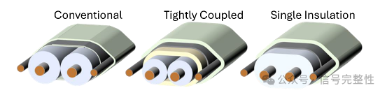
Figure 1: Different Twinax Designs
One of the largest contributors to skew is the conductor not being perfectly centered in the insulation. This is measured in percentage with 100% being perfectly centered. See Figure 2 [1]. This parameter can also be described as eccentricity (opposite of concentricity). Eccentricity is normally measured in microns and is a measure of the off-center position. The skew will vary depending on the off-center position and rotation within the twinax. See Figure 3. These positions cannot be controlled in the manufacturing process. As a result, the positions are pseudo-random. To understand skew variation requires many samples and statistical methods. See Figure 4. This shows skew levels at discrete concentricity values. Note that in each case the skew varies between some low value and a maximum value. The maximum value follows the concentricity. Higher concentricity equals lower skew.
Tightly coupled twinax with an extruded 2nd insulation or Single Extrusion Twinax (see Figure 1) also need to be concentric. Any deviation from concentricity will similarly result in skew.
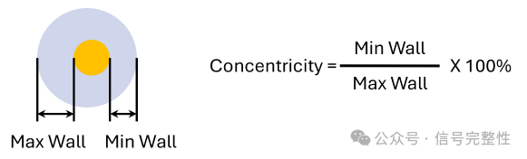
Figure 2: Definition of concentricity
Figure 3: Examples of concentricity/eccentricity position and rotation
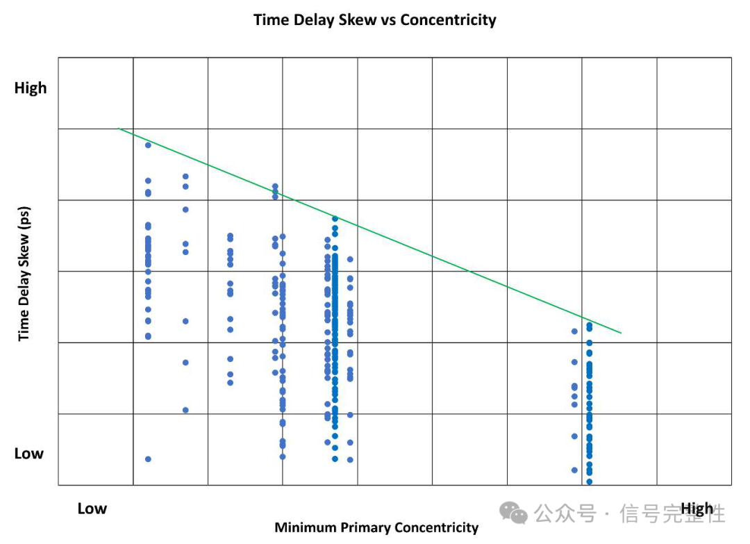
Figure 4: Range of skew values for discrete concentricity levels
Due to variations in tooling and gravity, the insulation shape is never perfect. In the case of round extrusion, this is called ovality. Figure 5. It is the difference between the largest and smallest cross-sectional dimension and measure in um. 0um is perfect. Similar to concentricity, ovality causes the signal conductor to be in an off-center position in a pseudo-random variation.
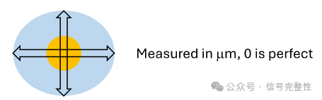
Figure 5: Picture of ovality
Twinax cables commonly have longitudinal and spiral or helically wrapped tapes for shielding, insulation and outer covering or jacket. These tapes help to optimize and control signal integrity properties as well as mechanical stability. Shields are typically longitudinally wrapped. See Figure 6. The red dotted line represents the edge of tape wrap. Other tapes are normally helically wrapped. See Figure 7. Typical defects that can cause skew are non-uniform tightness or deformation of thickness. See Figure 8 [1] and Figure 9. Longitudinal wrapping is most susceptible to non-uniformities. A non-uniform wrapping tightness will cause skew that is random and difficult to predict. Deformation of thickness is most likely to be caused by helical wrapping or an extruded secondary insulation. Deformation of thickness for a second insulation layer has an effect similar to concentricity.
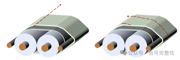
Figure 6: Longitudinal Wrap Figure 7: Helical Wrap
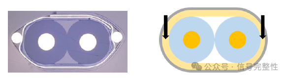
Figure 8: Non-uniform tightness Figure 9: Deformation of Thickness
Dimensional variation also contributes to skew. Even small variations in dimensions like conductor or insulation OD will increase time delay skew. Figure 10 shows that even a 1% OD variation can cause a noticeable increase in skew. In this simulation, plus and minus 1% OD variation is added to a twinax with 97% worst-case concentricity. The skew increase depends on frequency and is nearly a 50% increase at low frequency. In the time domain, the skew increases about 45% with a 15ps rise-time.
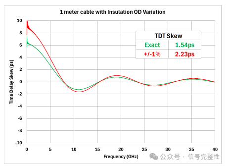
Figure 10: Example of 1% OD Variation
Most skew cause mechanisms are not fixed or constant with length. This will cause a non-uniform behavior of skew as noted in the next section.
Behavior of Time Delay Skew
The common frequency domain behavior of twinax skew is similar in shape to a Sinc function. The skew starts at a high level at low frequency (near DC) approaches and passes through zero skew, then oscillates around a fixed magnitude. The magnitude of the oscillations decreases with increasing frequency. See example of simulated skew and measured skew in Figure 11 and Figure 12.
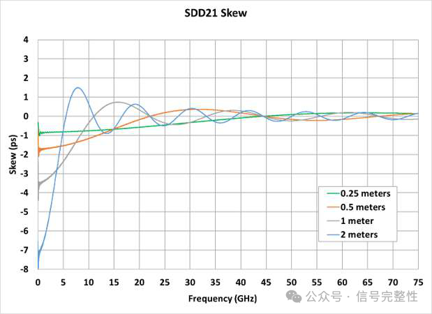
Figure 11: Twinax Skew vs Length Simulation
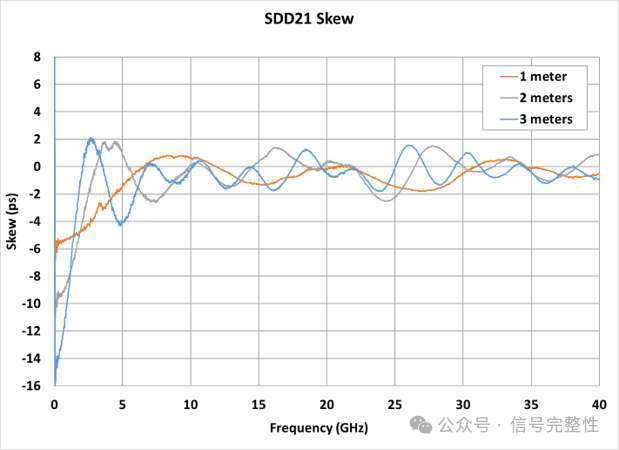
Figure 12: Twinax Skew vs Length Measurement
The cause of the decreasing/oscillating skew behavior is the within pair coupling between the Positive and Negative signals. The coupling between P & N is like crosstalk. Only it’s good crosstalk. Part of P couples to N and part of N couples to P. This gradually makes the phase of P & N more alike. The coupling tends to reduce skew with increasing frequency. The higher the frequency, the stronger the coupling resulting in a lower skew. The within pair coupling and its effect on skew is easiest to see in the time domain. Figure 13 shows the Time Domain Transmission (TDT) components of the differential signal. The naming of the differential components uses even-odd port mapping. See Figure 14 for a diagram of the four signal components. Note that at the rising signal edges there is strong coupling. TDT23 and TDT41 have a peak due to the high frequency content and then decay. It should be noted that TDT23 and TDT41 are difficult to distinguish because they have nearly the same magnitude. Figure 13 also shows that the coupling components reduce skew. The skew between the differential components of TDT21-TDT23 and TDT43-TDT41 (with coupling) is much lower than the TDT21 vs TDT43 skew. Single-ended skew measurements are not an accurate representation of P to N skew in a differential system. Including the coupling components is essential.
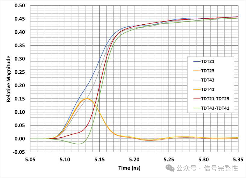
Figure 13: TDT Components
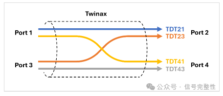
Figure 14: Diagram of TDT Signal Components
The sinc-like oscillations are a result of different propagation speeds in the twinax. Differential mode and common mode commonly have different propagation speeds. When the speeds or time delays result in a 180-degree phase shift, newly generated skew along the length of the cable negates previous skew and causes a null. This occurs at a frequency of 1/(2*|common mode delay-differential mode delay|) and all integer multiples. See Figure 12 and Figure 15. In this example, the 3 meter long cable has a differential to common mode delay difference of about 260ps. This causes a first null around 2GHz. It should be noted that the null may not be at exactly zero skew due to any lumped skew as noted later in the paper.
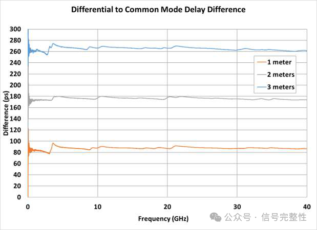
Figure 15: Differential vs Common Mode Delay for Figure 12
Twinax skew is often quoted as a value per meter. This is not accurate. Skew is not linear with length. This is due to two reasons. The first is due to manufacturing variation. Skew cause mechanisms are not constant with length. Therefore, ½ of the twinax does not have ½ of the skew. The second reason is that the within pair coupling tends to reduce skew over length. Similar to the reduction of skew with increasing frequency, a longer twinax means more coupling. Referring to Figure 11 & Figure 12, note that near DC, the skew is linear with length. For example, the skew in Figure 12 is approximately 5ps, 10ps and 15ps at 1, 2 & 3 meters. Note there is a small amount of error due to some lumped skew in the measurement system. The simulation in Figure 11 shows a more exact correlation with length. At very low frequency, the skew is linear with length due to very weak within pair P to N coupling. At higher frequencies, the relationship is no longer linear. This is easiest to see in the time domain. Figure 16, Figure 17 and Figure 18 show the time domain skew for the twinax examples in Figure 11 and Figure 12. Note in Figure 17 and Figure 18 that the 2 meter skew is not double 1 meter and 3 meter is not triple 1 meter. In both cases it is lower due to more within pair coupling in the longer length. This is also true for Figure 16 for lengths of 0.25 meter to 1 meter. 2 meters does not follow this same trend. This cable has higher insertion loss. This causes the spectral content of the TDT step response to shift lower in frequency where skew is higher. This can be seen in Figure 19. Note that the rise-time of the output of the 2 meter cable has slowed significantly. Although this is an extreme example, it shows another example of why skew is not linear with length.
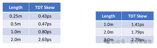
Figure 16: Time Domain for Figure 11 Figure 17: Time Domain for Figure 12
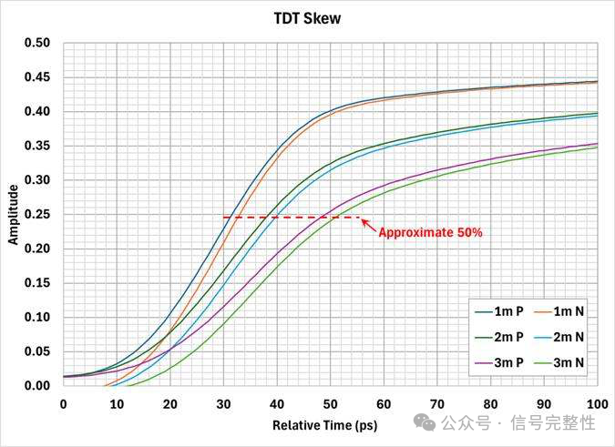
Figure 18: TDT Skew for Figure 17
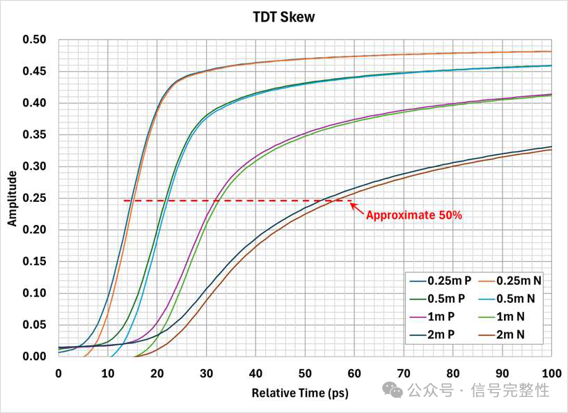
Figure 19: TDT Skew for Figure 16
As noted earlier, the skew cause mechanisms are not constant through a length of twinax. This causes the skew of subsequent pieces of the same length to be different. See Figure 20 and the associated cutting diagram Figure 21. This shows the results for a 4 meter twinax that was first cut into two 2 meter twinax and then to four 1 meter twinax. The two 2 meter and four 1 meter lengths do not match each other. Both the frequency domain and time domain skew vary along the length. In addition, the sum of the individual TDT values do not add to arrive at the longer length. This is due to the twinax loss affecting the spectral content and the within pair coupling of short vs long cables as noted earlier.
Figure 20: Skew Measurements for Twinax Cut per Figure 21
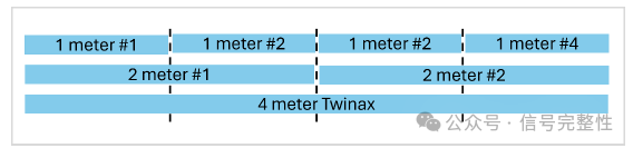
Figure 21: Twinax Cutting Diagram for Figure 20
Intuitively, skew would seem to be independent of transmission direction. This is often not the case. Lumped skew before or after the twinax or skew varying within the twinax length will cause SDD21 skew and SDD12 skew to be different. See a simulation with lumped skew in Figure 22. In this example, 1ps of fixed skew is added before 1 meter of twinax. In the SDD21 direction, the fixed skew is at the drive end. This causes the frequency domain skew to have larger amplitude oscillations, but the oscillations are still around a skew of zero. The TDT skew in the same direction is almost the same as without the fixed skew. This is due to the within pair coupling tending to reduce the added skew over the length of the twinax. In this case, the within pair P to N coupling nearly eliminates the added skew. This reduction will be situation dependent based on the amount of lumped skew, cable length and twinax design. In the SDD12 direction (fixed skew after the twinax), the frequency domain skew now oscillates around a bias of the 1ps of lumped skew. The TDT skew is 1ps higher than the twinax alone. Figure 23 shows the same behavior for measured skew in a cable assembly that had lumped skew on the ends.
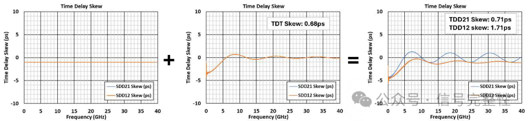
Figure 22: Twinax with Proceeding Lumped Skew
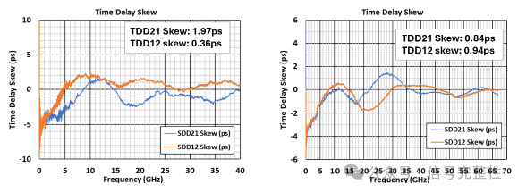
Figure 23: Lumped Skew Measured Figure 24: Twinax with Skew Variation
Figure 24 shows an example of the directional behavior caused by skew variation within the twinax. Generally, skew variation in twinax changes the frequency domain shape but has less effect on skew over a wide frequency range. In this example, note that both the SDD21 and SDD12 skew deviate from the normal decaying oscillations and reach a second peak at 28 GHz and 22 GHz respectively. A second peak is common for twinax with skew variation along its length. In this case, the skew is relatively low and has minimal impact. Another example in Figure 25 shows the secondary peaks occurring at higher frequency. There is little effect on the difference between SDD21 and SDD12 in the time domain. In this case, there is a different effect on signal integrity. The combination of higher frequency and slightly higher skew causes an increase of insertion loss. See Figure 26.
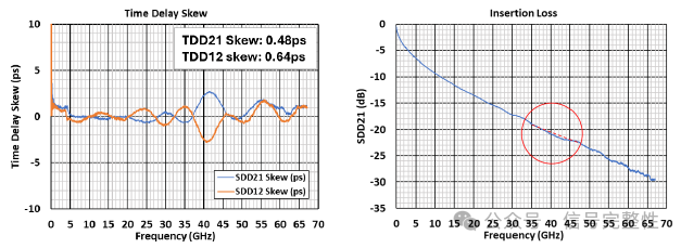
Figure 25: Skew Variation Example 2 Figure 26: SDD21 for Figure 25
Skew Mitigation Strategies
All skew in twinax is caused by manufacturing variation. An important mitigation strategy is precise control of the manufacturing process and material inputs. This is an ongoing process for most twinax manufacturers, but not the focus of this paper. The mitigation strategies in this paper assume a high level of control and identify design-related mitigation strategies.
As noted earlier, the coupling between P & N signals within the twinax reduces skew over length and as frequency increases. Using tight coupling to increase the P to N coupling level can help to reduce skew. Percent coupling is defined as the coupling between signal lines as compared to total coupling including between signal lines and the shield. It can be calculated from the differential and common mode impedance. See Figure 27 [2]. Figure 28 and Figure 29 show the simulated skew for 3 cable designs. All for the same nominal twinax except for coupling level. Each simulation includes the exact same level of conductor eccentricity to generate skew and is for a 1 meter long twinax. Note that the skew drops significantly with increased coupling. For reference, Figure 30 shows the TDT representation of the increased coupling (T23/T41).
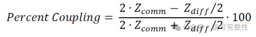
Figure 27: Percent Coupling Calculation
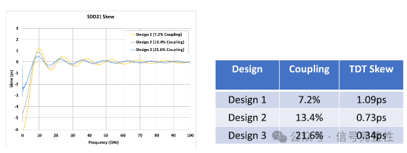
Figure 28: Skew vs Coupling % Figure 29: Skew vs Coupling %
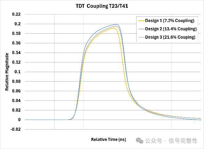
Figure 30: TDT Coupling for Figure 29
The oscillating behavior of the frequency domain skew can be controlled to reduce skew.
As described previously, the oscillating behavior repetition rate is dependent on the difference between differential and common mode time delay. Designing the twinax to increase the time delay difference will cause the skew to dampen/reduce earlier in frequency. See the simulations in Figure 31, Figure 32 and Figure 33. As the time delay delta is increased from 20ps to 45ps and then to 75ps, the frequency domain skew peaks earlier then dampen sooner. There is also a significant reduction in time domain skew. Figure 34 shows the time domain coupling for T23/T41. Note that the time length of the coupling signal increases as the difference between differential and common mode delay increases. The longer length creates stronger coupling helping to reduce skew. Note that the length of the coupling signal from bottom to peak is equal to the difference between differential and common mode delay.
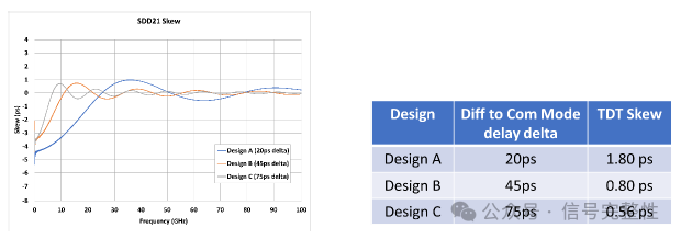
Figure 31: Frequency Skew vs Delay delta Figure 32: TDT Skew vs Delay delta
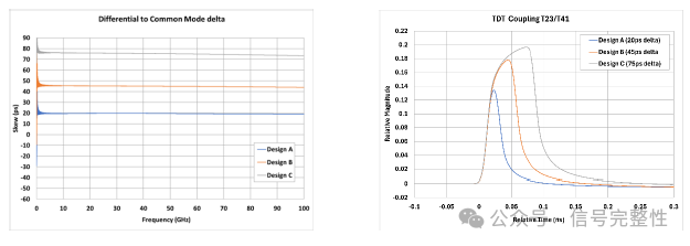
Figure 33: Delay delta for Figure 31/32 Figure 34: TDT Coupling Figure 31/32
See Figure 35-38 for measured data with different differential vs common mode delay differences. Twinax 1 has a difference of 56ps in this 1 meter cable. Twinax 2 has a difference of about 1.5ps (nearly zero). The skew is significantly higher in twinax 2. Note in Figure 38 that there is very little P to N coupling in Twinax 2. Figure 36 shows that when differential and common mode delay are the same or nearly the same, there is no oscillating behavior in the frequency domain. The skew is close to a constant value at all frequencies. This type of skew pattern is likely to have a larger effect on very high data rate signals.
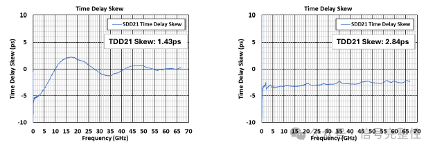
Figure 35: Twinax 1 Skew Figure 36: Twinax 2 Skew
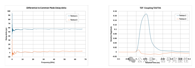
Figure 37: Delay delta for Twinax 1 & 2 Figure 38: TDT Coupling Twinax 1 & 2
Skew Under Thermal & Bending Conditions
In well-designed and manufactured twinax cables, time delay skew is relatively stable over normal operating temperatures. High temperatures have little effect on skew. Extreme low temperatures do affect skew. See example in Figure 39 and Figure 40. This data is for a thermal cycling test on a 30 AWG 112G twinax cable. From 25C to 85C and back down to -20C. There is little effect on skew. There is some variation likely due to measurement variation and there is a low frequency improvement at -20C, that affects TDT, but has little effect at high frequencies. The only big change is at -40C. The frequency domain oscillations become larger and the TDT skew changes sign due to a larger low frequency oscillation. The -40C behavior is common in high-speed twinax cables. It is caused by the difference in the thermal expansion/contraction rates of the different materials used in the twinax. As an example, metals and plastics have very different expansion rates. The good news is that in a well-made cable, the change at extreme low temperature (-40C) is not permanent. See Figure 41 This is the 25C data at 3 time points. Test 1 before any thermal cycling, Test 5 after 85C and before 0C, Test 9 after -40C. All 3 25C measurements match very closely. In the case of this cable, -40C is likely OK for transportation or storage. Operating at -40C would require further verification.
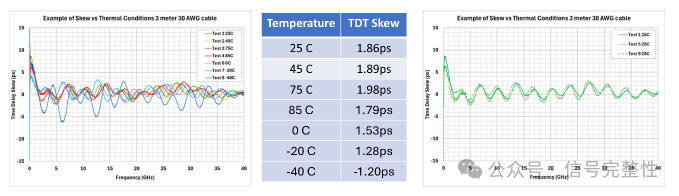
Figure 39: Skew vs Temperature Figure 40: TDT Figure 41: Skew thermal stability
Bending and routing can have a negative effect on skew. The predominant effect is in the frequency domain. The effect on time domain skew is less. See Figure 42. This is 112G 2-meter long twinax in a 16 pair bundle for a DAC cable assembly. Test 1 is the cable in a loose loop with no stresses. Test 2 is the same cable routed in a fixture to simulate an installed cable. The installation simulation has four 90 degree bends and one 180 degree bend. All bending radii are small compared to industry norms. Test 2 causes the frequency domain oscillations to get slightly larger. There is only a small effect on time domain skew. In this case, it gets slightly lower. This is the normal behavior for a well-made twinax. There are only small effects from bending. Test 3 adds torsion in addition to bending. Two 360 degree twists were applied to the same cable before routing in the fixture. Two full twists is extreme compared to a normal installation, but is meant to clearly demonstrate the effect of torsion. The frequency domain oscillations increase significantly with the added torsion. Through numerous similar tests and different cables, it has been found that torsion (twisting) has a larger effect on skew than bending. In Test 3, time domain skew again has minimal change. The increased magnitude frequency domain oscillations can have a negative effect on insertion loss. See insertion loss for the same tests in Figure 43. Note that the insertion loss has very little change from the smaller oscillations caused by bending. When torsion is added in Test 3, the larger skew swings at 25-28GHz and 31-36GHz cause increased insertion loss. This is the most common negative signal integrity effect of cable routing.
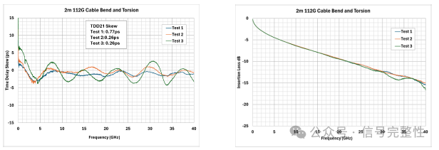 Figure 42: Skew with Bend & Torsion Figure 43: SDD21 Loss with Bend / Torsion
DAC Measurement Results
In this section, we empirically examine cable bend stress impact on skew and BER performance on OSFP cable assemblies. The results here expand on the work previously done by Farrahi [3], Lai [4], and Moon [5] to show the relationship between skew and actual BER measurements. Here, we will further take into account the impact of cable bend stress on skew and BER which can be significant as demonstrated by Tooyserkani[6] in the case of skew on OSFP-800G cable assemblies. As discussed in previous sections, this bend stress is magnified as data rate per lane doubles to 200G due to the increased sensitivity to cross-sectional asymmetries and deformations with the halving of the wavelength.
The test setup used to induce bend stress on cable assemblies is shown in Figure 44a below. This apparatus is used to subject the cable to an initial 90° bend, followed by a 180° bend, another 90° bend, and finally a sharp 180° pinch in the middle of the cable after which the bend sequence is reversed. A key objective of these measurements is to associate the amount of skew to BER. Thus, for a given bend stimulus, great care is taken to not perturb the bend-induced skew on a cable between its S-parameter measurement and corresponding BER measurement. Towards this end, each skew and its accompanying BER measurement for a given differential pair are taken immediately after each other with no disturbance of the DUT other than to unplug from one set of OSFP receptacles (on the SerDes evaluation board) to the other OSFP receptacles (on the MCB).
The SerDes uses standard initialization and adaptation routines – no custom manual tuning are used in these measurements. The transmit and receive SerDes are different ICs with independent reference clocks, to represent the clock recovery challenges in a real link, as opposed to a simpler self-loopback configuration.
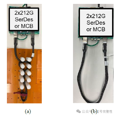
Figure 44: Setup for OSFP cable assembly when connected to the SerDes test board in (a) bend stress state and (b) relaxed state.
To start, Figure 45 shows the insertion loss of three OSFP cable assemblies which are used throughout this section. In each case, all 16 differential pairs in the cable are examined. Figure 45a is for a 1m OSFP cable assembly originally designed for 800G. The blue curves represent insertion losses for the relaxed (i.e. no tight bends) condition of the cable assembly. The red curves represent the insertion loss when they are subject to the bend stress in Figure 44. The response (even under the bent state) is very good up to 26GHz Nyquist but insertion loss variation starts to become evident around 40GHz, particularly when bent.
Figure 45b is for a 1m OSFP-1.6T cable assembly. Not surprisingly, because the cable was designed for high bandwidth, the performance is better past 26GHz out to 53GHz for not only the straight condition but also the bent condition where the variation is significantly improved. The variation is reasonably controlled out to the 67GHz limit of the VNA. As discussed in previous sections, this improvement comes from not only a higher bandwidth cable design but also deliberate design considerations targeted to improve robustness under bend stress.
Figure 45c is for a 1.2m OSFP-1.6T cable assembly based on the same design as the 1m OSFP-1.6T cable in Figure 45b. At this longer length, some variation is noticeable at Nyquist, but as will be seen later, this is still well-managed by the robustness of the SerDes and its ability to adapt to changes in the channel.
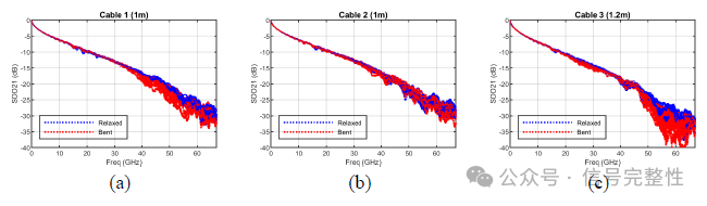
Figure 45: Insertion loss of the differential pairs in an OSFP cable assembly: (a) 1m OSFP-800G, (b) 1m OSFP-1.6T, and (c) 1.2m OSFP-1.6T under straight (blue) and bent (red) conditions.
To highlight the impact of bend stress on insertion loss, Figure 46 shows a scatter plot of the insertion loss at 53.125GHz Nyquist for each of the cable assemblies where the Y-axis shows the insertion loss under the bent condition and the X-axis shows the insertion loss for the relaxed condition. As suggested by Figure 45, the 1m OSFP-800G cable shows more loss induced by the bend compared to the higher speed 1m OSFP-1.6T cable by its tendency to exhibit points below the identity reference line representing no change in loss.
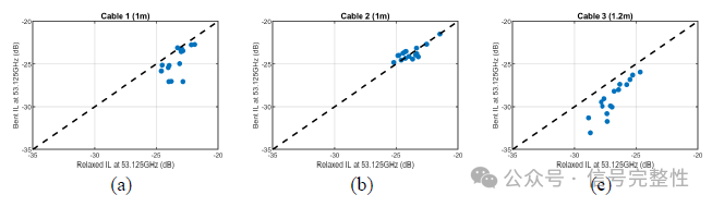
Figure 46: Scatter plot of insertion loss at 53.125GHz for unstressed/straight condition vs the bent condition. (a) 1m OSFP-800G, (b) 1m OSFP-1.6T, and (c) 1.2m OSFP-1.6T.
Having examined the cable losses in Figures 45 and 46, we now examine the skew of these cables. Figure 47 shows the skew spectrum for each of the cables. Again, this is shown for both the straight condition (blue) along with the bent condition (red). Looking at Figures 47a and 47b, two prominent features deserve mention. First, the overall skew of the 1.6T design is lower than that of the 800G design, as would be expected for a higher fidelity SI design. Second, the 800G design in Figure 47a shows a considerable increase in skew around 40-50GHz under the bend state. Even though the relaxed cable skew is higher in absolute picoseconds at lower frequencies, one should keep in mind the increased sensitivity at higher frequencies due to the relatively smaller associated unit-interval with this frequency content. Thus, it is comforting to see the lack of skew-increase near Nyquist in the higher speed designed cable in Figures 47b and 47c.
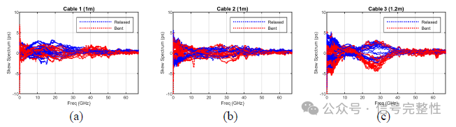
Figure 47: Skew spectrum of OSFP cable assemblies: (a) 1m OSFP-800G, (b) 1m OSFP-1.6T, and (c) 1.2m OSFP-1.6T under straight (blue) and bent (red) conditions.
Figures 45-47 have shown the effects of bending on s-parameter based characterizations of the cables, but what is ultimate concern is the link error rate in application. Towards this end, we look at the BERs measured with the 212G SerDes evaluation board shown in Figure 44a. The link is run with all lanes active (i.e. including crosstalk effects) carrying PRBSQ-31 framed data with BERs measured over 60-second intervals. For all the cables, BER remains better than 10-8 even in the bent state, never encountering a framing error in any case. Even though an SI improvement was generally apparent in the s-parameters of the new OSFP-1.6T cable design, the Serdes was able to yield good BER in all cases. We attribute this to the strength of SerDes. A 10-8 BER is a good result. The filtering in the SerDes was able to largely adapt to the channel variation associated with the bend to the point where it was “in the noise” of a 10-8 BER level. The authors believe that if longer, more stressful cables were used in the comparisons, then the 800G and 1.6T cable constructions would exhibit BER differences between the relaxed and bent states. This will be further studied in the future.
Conclusions
This paper has explored intra-pair skew as an SI characteristic of DAC twin-ax cables for 224G applications. Skew is a means to assess the imbalanced phase of a differential channel and is a different means to assess mode conversion. Skew and mode conversion fundamentally arise from P-N asymmetries or nonuniform construction in the twin-ax cable. Characterizations of such deformations include ovality, concentricity, and dielectric thickness due to taping tension variation. Skew is not additive along the length of a cable nor is it uniformly distributed along the cable. The contributions of skew can be erratically distributed (commensurate with the unintended asymmetries) along the cable and they can combine either constructively or destructively.
Clearly, an obvious step in controlling skew is minimizing variation in manufacturing to ensure tight symmetry. But the cable design should also keep in mind that asymmetries will be introduced in the field when cables are subject to physical stresses such as bending or twisting. We have described methods to minimize the induced skew in such cases by considering the impact of the different propagation velocities of the differential and common modes and using this to our advantage to minimize skew.
Finally, results were shown on full OSFP cable assemblies which were subject to significant bend stresses. By employing the practices promoted here, the skew of the cables was well behaved even when subject to stress. Furthermore, a good BER was maintained in such conditions. We consider such practices vital to producing robust, high-quality cable assemblies as the industry migrates to the more SI sensitive 224G applications.
Acknowledgements
The authors wish to thank; Huanzhong Yan for all of the twinax testing, data and collaboration for testing method and fixture development. Andy Nowak for his work in test method and fixture development.
We would also like to express our gratitude to the Broadcom team for their invaluable support in collecting data for this paper.
References
[1] Jiang, et al., “Tutorial OSFP/QSFP DD112G PAM4 Channel for 800G System Applications”, DesignCon 2022
[2] Casher, Patrick, “Materials Used in Gigabit Cable and Their Electrical Characteristics”, DesignCon 2018
[3] Farrahi, et al., “Does Skew Really Degrade SERDES Performance”, DesignCon 2015.
[4] Lai, et al., “Skew Metric and BER Testing Correlation for NRZ/PAM4 Signaling”, DesignCon 2019.
[5] Moon, et al., “Effective Intra-Pair Skew, EIPS and Intra-Pair Skew Modeling Method”, DesignCon2022.
[6] Tooyserkani, et al., “The Case for 36 dB C2M Insertion Loss at 200G”, Plenary 802.3dj, Nov. 2023.
相关阅读:
|
PCIe6.0 PCB对内Skew的延迟补偿方法 [DesignCon最佳论文推荐] 224G PAM4 线性系统:主机TxRx、电光通道特性及端到端链路仿真与分析 [DesignCon最佳论文推荐]224G BGA Pinmap及过孔的创新设计 [DesignCon最佳论文推荐]研究PCB 制造变化致引脚区域串扰的恶化-Intel 224G通道的PCB制造技术及公差控制对信号完整性的影响 如何从仿真的世界看串扰 【干货】高速电路中串扰引发的损耗问题 |
 |
 |