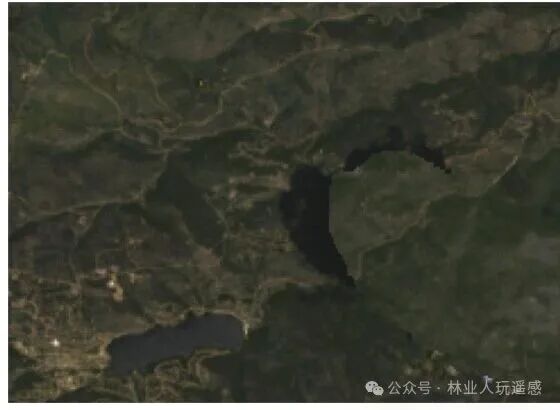
“ The rioxarray package is used to read, cloud-remove, and fill pixels in Landsat data.”
01
—
Data Reading and Display
This section discusses the rioxarray package for processing Landsat data. The example data uses the cold-spring-fire dataset from the earthpy package, which can be downloaded directly via the earthpy package or accessed from the earthpy data repository:
https://ndownloader.figshare.com/files/10960109
If you still cannot download, you can use the following link:
https://pan.baidu.com/s/1bAnUo0S_ojxXdkyBqWAnLg?pwd=gxu2 Extraction code: gxu2
import os
from glob import glob
import matplotlib.pyplot as plt
import numpy as np
import xarray as xr
import rioxarray as rxr
import earthpy as et
import earthpy.plot as ep
data = et.data.get_data("cold-springs-fire")# If you download the data locally by other means, modify the path according to the storage location
# The data downloaded by earthpy is stored by default in et.io.HOME, which can be checked with print(et.io.HOME)
os.chdir(os.path.join(et.io.HOME, "earth-analytics", "data"))
landsat_post_fire_path = os.path.join("cold-springs-fire", "landsat_collect", "LC080340322016072301T1-SC20180214145802", "crop")
post_fire_paths = glob(os.path.join(landsat_post_fire_path, "*band*.tif"))
post_fire_paths.sort()
post_fire_paths['cold-springs-fire\landsat_collect\LC080340322016072301T1-SC20180214145802\crop\LC08_L1TP_034032_20160723_20180131_01_T1_sr_band1_crop.tif', 'cold-springs-fire\landsat_collect\LC080340322016072301T1-SC20180214145802\crop\LC08_L1TP_034032_20160723_20180131_01_T1_sr_band2_crop.tif', 'cold-springs-fire\landsat_collect\LC080340322016072301T1-SC20180214145802\crop\LC08_L1TP_034032_20160723_20180131_01_T1_sr_band3_crop.tif', 'cold-springs-fire\landsat_collect\LC080340322016072301T1-SC20180214145802\crop\LC08_L1TP_034032_20160723_20180131_01_T1_sr_band4_crop.tif', 'cold-springs-fire\landsat_collect\LC080340322016072301T1-SC20180214145802\crop\LC08_L1TP_034032_20160723_20180131_01_T1_sr_band5_crop.tif', 'cold-springs-fire\landsat_collect\LC080340322016072301T1-SC20180214145802\crop\LC08_L1TP_034032_20160723_20180131_01_T1_sr_band6_crop.tif', 'cold-springs-fire\landsat_collect\LC080340322016072301T1-SC20180214145802\crop\LC08_L1TP_034032_20160723_20180131_01_T1_sr_band7_crop.tif']Next, we will first use the .squeeze() method to open a single band, ensuring that the output xarray object has only 2 dimensions instead of 3.
band_1 = rxr.open_rasterio(post_fire_paths[0], masked=True).squeeze()
band_1.shape  # (177, 246)
We will plot the image of one of the bands.
f, ax = plt.subplots()
band_1.plot.imshow(ax=ax, cmap="Greys_r")
ax.set_axis_off()
ax.set_title("Plot of Band 1")
plt.show()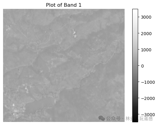 The following code will stack each band we opened into a new single output array, but this method is only efficient when we want to process all bands in the data. Considering the size of Landsat data, we may also need to remove unwanted bands.
all_bands = []
for i, aband in enumerate(post_fire_paths):
    all_bands.append(rxr.open_rasterio(aband, masked=True).squeeze())
    all_bands[i]["band"] = i + 1
Convert the list of bands into a single xarray object.
landsat_post_fire_xr = xr.concat(all_bands, dim="band")Let’s take a look at the data.
landsat_post_fire_xr.plot.imshow(col="band", col_wrap=3, cmap="Greys_r")
plt.show()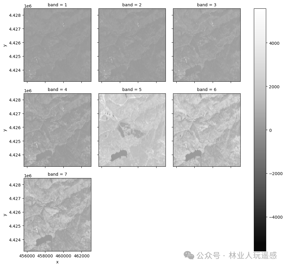 We can use the ep.plot_rgb() function from the earthpy library to plot a 3-band color composite image of Landsat.The ep.plot_rgb() function requires:
- A numpy array containing the bands we want to plot. We can obtain this array using xarray_name.values, which should follow the band order of xarray (bands first);
- The numerical positions of the bands we want to plot in the array;
ep.plot_rgb(landsat_post_fire_xr.values, rgb=[3, 2, 1], title="RGB Image")
plt.show()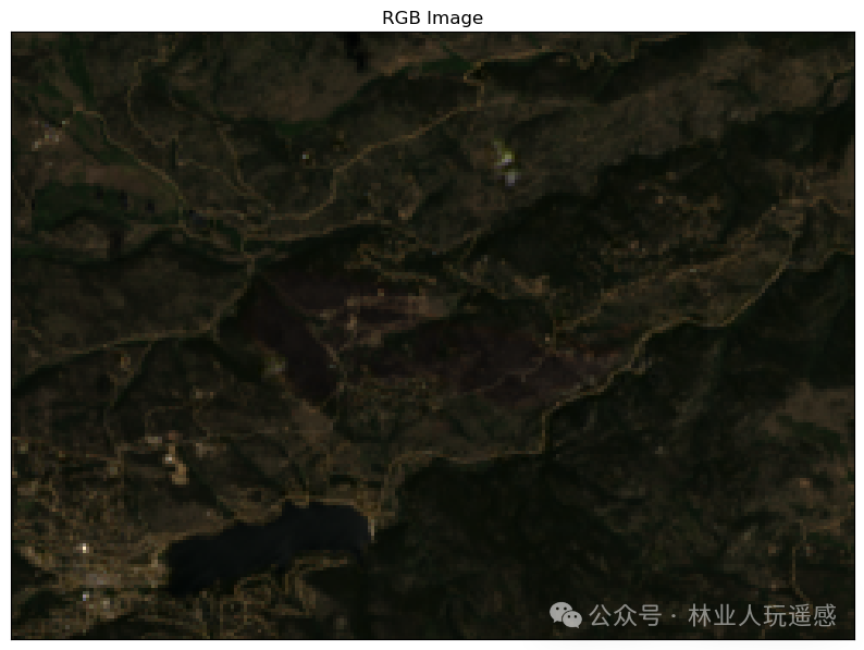 This image appears darker; we can use the stretch parameter built into the plot_rgb() function to stretch the image, and the str_clip parameter allows you to specify the proportion of data to truncate from the tail. The larger this value, the more the data is stretched or brightened.
ep.plot_rgb(landsat_post_fire_xr.values, rgb=[3, 2, 1], title="RGB Image-Linear Stretch", stretch=True, str_clip=1)
plt.show()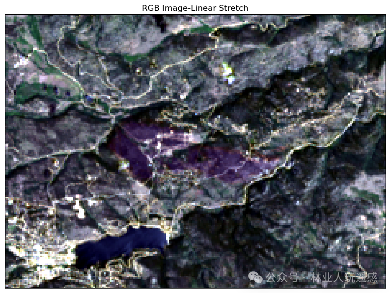 We can create a histogram to view the distribution of pixel values in the plotted RGB bands.
band_titles = ["Band 1", "Blue", "Green", "Red", "NIR", "Band 6", "Band 7"]
ep.hist(landsat_post_fire_xr.values, title=band_titles)
plt.show()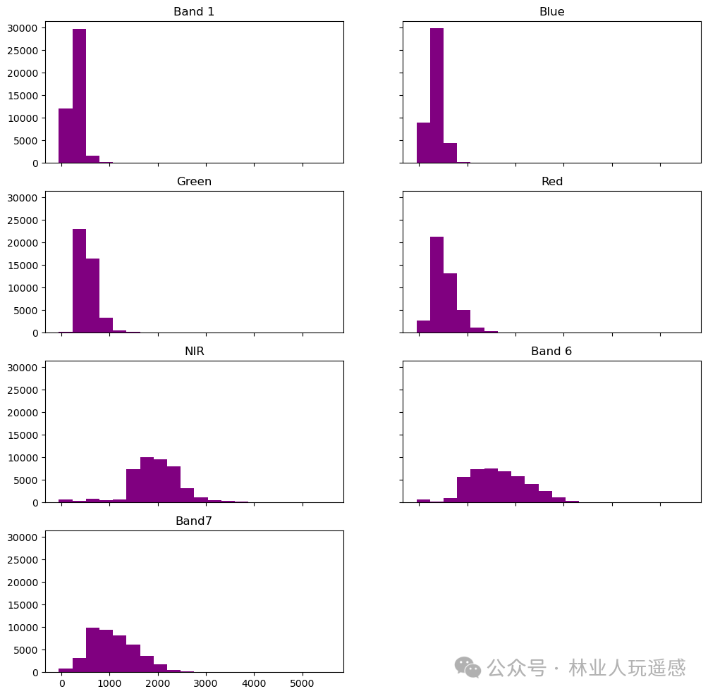 We create a CIR image using Landsat bands 4, 3, and 2.
ep.plot_rgb(landsat_post_fire_xr.values, rgb=[4, 3, 2], title="CIR Landsat Image", figsize=(10, 10))
plt.show()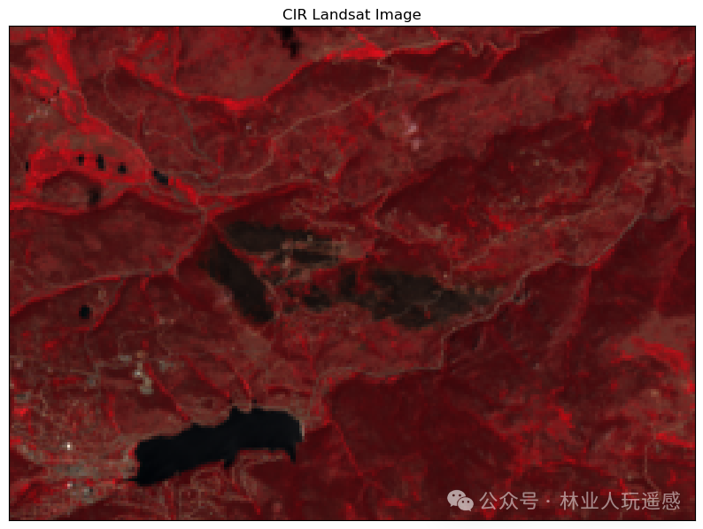
02
—
Cloud Removal in Imagery
We first define two functions, open_clean_band and process_bands. These functions are used to open single-band stored Landsat imagery and stack them into a multi-band image.
def open_clean_band(band_path, crop_layer=None):
    if crop_layer is not None:
        try:
            clip_bound = crop_layer.geometry
            cleaned_band = rxr.open_rasterio(band_path, masked=True).rio.clip(clip_bound, from_disk=True).squeeze()
        except Exception as err:
            print(err)
    else:
        cleaned_band = rxr.open_rasterio(band_path, masked=True).squeeze()
    return cleaned_band

def process_bands(paths, crop_layer=None, stack=False):
    all_bands = []
    for i, aband in enumerate(paths):
        cleaned = open_clean_band(aband, crop_layer)
        cleaned["band"] = i + 1
        all_bands.append(cleaned)
    if stack:
        return xr.concat(all_bands, dim="band")
    else:
        return all_bands
Then, we will load and plot the Landsat data. We will only use the RGB (Red, Green, Blue) bands and the NIR (Near Infrared) band, and we can filter the required bands using *band[2-5]*.tif in glob.
landsat_dirpath_pre = os.path.join("cold-springs-fire", "landsat_collect", "LC080340322016070701T1-SC20180214145604", "crop", "*band[2-5]*.tif")
landsat_paths_pre = sorted(glob(landsat_dirpath_pre))
landsat_pre = process_bands(landsat_paths_pre, stack=True)
ep.plot_rgb(landsat_pre.values, rgb=[2, 1, 0], title="Landsat Image")
plt.show()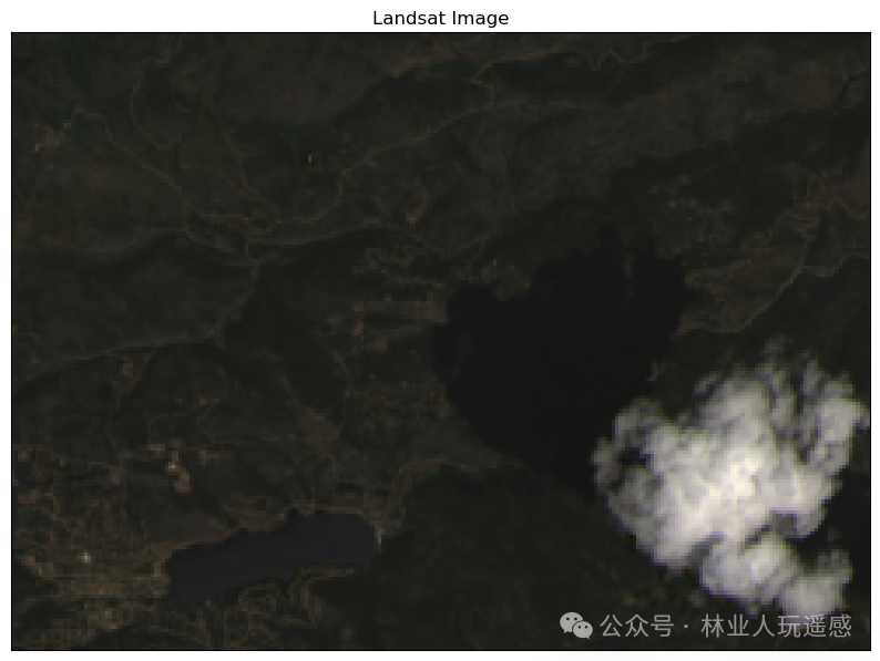
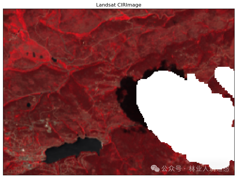
We see that there is a large cloud in our image. This cloud will affect any quantitative analysis we perform on the data. We can use a cloud mask layer to identify pixels that may be clouds or cloud shadows. Then, we set these pixel values to masked status so that they are not included in calculations during quantitative analysis.
We mention that a “mask” refers to a layer that “turns off” pixel values in raster data that we do not want to include in the analysis or sets them to NaN (Not a Number).
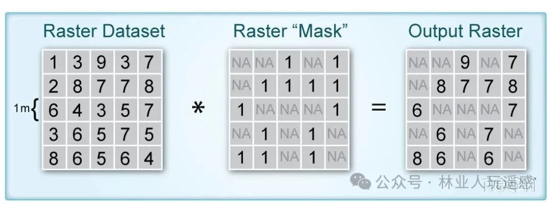
Many remote sensing datasets come with quality layers that we can use as masks to eliminate unwanted pixels (such as cloud pixels). For example, in Landsat data, such mask layers can identify pixels representing cloud cover, cloud shadows, or even water bodies. When we download Landsat 8 data, the data includes a processed cloud shadow/mask raster layer, which is named in the format “xxx_pixel_qa.tif”. In the example data we are using, the name of this layer is:
LC08_L1TP_034032_20160707_20170221_01_T1_pixel_qa_crop.tif
We first use rioxarray to open this pixel_qa layer and plot its image.
landsat_pre_cl_path = os.path.join("cold-springs-fire", "landsat_collect", "LC080340322016070701T1-SC20180214145604", "crop", "LC08_L1TP_034032_20160707_20170221_01_T1_pixel_qa_crop.tif")
landsat_qa = rxr.open_rasterio(landsat_pre_cl_path).squeeze()
high_cloud_confidence = em.pixel_flags["pixel_qa"]["L8"]["High Cloud Confidence"]
cloud = em.pixel_flags["pixel_qa"]["L8"]["Cloud"]
cloud_shadow = em.pixel_flags["pixel_qa"]["L8"]["Cloud Shadow"]
all_masked_values = cloud_shadow + cloud + high_cloud_confidence

landsat_pre_cl_free = landsat_pre.where(~landsat_qa.isin(all_masked_values))
fig, ax = plt.subplots(figsize=(10, 8))
im = ax.imshow(landsat_qa.values, cmap="viridis")
ax.set_title("Landsat QA Layer")
cbar = fig.colorbar(im, ax=ax, fraction=0.03, pad=0.04)
cbar.set_label("Pixel QA Values")
plt.show()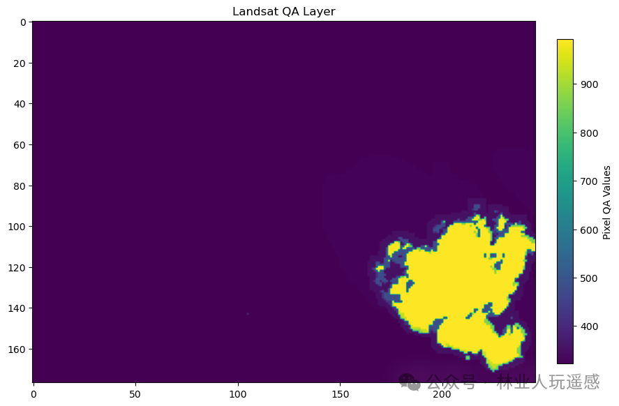
In the above image, we can see the cloud cover and its shadows. To address this issue, we need to directly mask or remove the cloud cover. To remove all pixels covered by clouds and shadows, we first need to determine what each value in the QA raster represents.
According to information provided by USGS, the meanings of values in the pixel_qa layer are as follows:
| Fill | 1 |
| Clear | 322, 386, 834, 898, 1346 |
| Water | 324, 388, 836, 900, 1348 |
| Cloud Shadow | 328, 392, 840, 904, 1350 |
| Snow/Ice | 336, 368, 400, 432, 848, 880, 912, 944, 1352 |
| Cloud | 352, 368, 416, 432, 480, 864, 880, 928, 944, 992 |
| Low confidence cloud | 322, 324, 328, 336, 352, 368, 834, 836, 840, 848, 864, 880 |
| Medium confidence cloud | 386, 388, 392, 400, 416, 432, 900, 904, 928, 944 |
| High confidence cloud | 480, 992 |
| Low confidence cirrus | 322, 324, 328, 336, 352, 368, 386, 388, 392, 400, 416, 432, 480 |
| High confidence cirrus | 834, 836, 840, 848, 864, 880, 898, 900, 904, 912, 928, 944, 992 |
| Terrain occlusion | 1346, 1348, 1350, 1352 |
In our example, we focus on Cloud Shadow, Cloud, and High confidence cloud, but in actual analysis, we may need to consider Medium confidence cloud and Low confidence cloud, depending on the specific analysis objectives.
We will reclassify the data based on the above values, using the xarray isin() function to create a mask, generating a binary cloud mask layer. In this mask, all pixels we want to remove or mask will be set to 1, and other pixels will be set to 0.
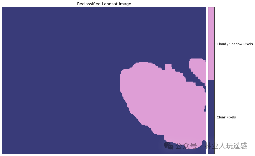
Next, we can complete the data masking process using the where() function. This function will apply the mask we created above to the xarray array. When applying the mask, ensure to prepend `~` to the mask inside the where() function. This must be done because the mask created by isin() has the positions we want to set to False as True, and vice versa. The `~` will flip all values in the array.
landsat_pre_cl_free = landsat_pre.where(~cl_mask)Alternatively, we can also directly input the mask values and pixel QA layer into the mask_pixels function. This is the simplest method for masking the data, but this function only accepts NumPy arrays, so we need to call the values method on all xarray data arrays (DataArray) used as input.
landsat_pre_cl_free = landsat_pre.where(~landsat_qa.isin(all_masked_values))
ep.plot_bands(landsat_pre_cl_free[3], cmap="Greys", title="Landsat Infrared Band", cbar=False)
plt.show()
ep.plot_rgb(landsat_pre_cl_free, rgb=[3, 2, 1], title="Landsat CIR Image")
plt.show()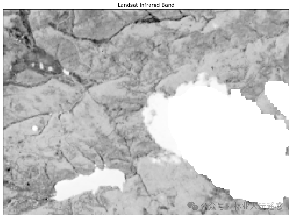
03
—
Filling Raster Values After Cloud Removal
Sometimes, a Landsat image may have many cloud pixels, and we want to replace or fill these pixels with pixels from another image.
We will still use the cold-spring-fire dataset for the example.
landsat_dirpath_pre = os.path.join("cold-springs-fire", "landsat_collect", "LC080340322016070701T1-SC20180214145604", "crop", "*band[2-4]*.tif")
landsat_paths_pre = sorted(glob(landsat_dirpath_pre))
landsat_pre = process_bands(landsat_paths_pre, stack=True)
To ensure the coherence of the processing, let me repost the relevant processing code from the previous section (with one variable name adjusted).
landsat_pre_cl_path = os.path.join("cold-springs-fire", "landsat_collect", "LC080340322016070701T1-SC20180214145604", "crop", "LC08_L1TP_034032_20160707_20170221_01_T1_pixel_qa_crop.tif")
landsat_qa = rxr.open_rasterio(landsat_pre_cl_path).squeeze()
high_cloud_confidence = em.pixel_flags["pixel_qa"]["L8"]["High Cloud Confidence"]
cloud = em.pixel_flags["pixel_qa"]["L8"]["Cloud"]
cloud_shadow = em.pixel_flags["pixel_qa"]["L8"]["Cloud Shadow"]
all_masked_values = cloud_shadow + cloud + high_cloud_confidence
landsat_pre_cl_masked = landsat_pre.where(~landsat_qa.isin(all_masked_values))
Plot the image to ensure that all cloud pixels have been removed.
ep.plot_rgb(landsat_pre_cl_masked, rgb=[2, 1, 0], title="Masked Landsat CIR Image")
plt.show()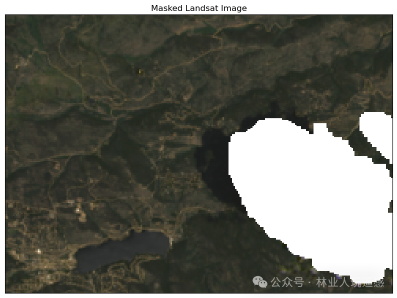
We have obtained a Landsat image with cloud pixels removed. To fill these pixels, we will replace them with pixels from another Landsat image of the same area and a similar time period.
We will read a cloud-free Landsat dataset from the same location.
Cloud-free Landsat data can be downloaded from the following link:
https://ndownloader.figshare.com/files/10960214?private_link=fbba903d00e1848b423e
cloud_free_path = os.path.join("cs-test-landsat", "*band[2-4]*.tif")
landsat_paths_pre_cloud_free = sorted(glob(cloud_free_path))
landsat_pre_cloud_free = process_bands(landsat_paths_pre_cloud_free, stack=True, crop_layer=clip_gdf)
In theory, we need to check whether the spatial extent and CRS of the two images are consistent, but in practical applications, we are definitely using the same scene image, so there should be no inconsistency in spatial extent or CRS.
We will use the where() function to implement the filling of raster values.
mask = landsat_pre_cl_masked.isnull()
landsat_pre_clouds_filled = xr.where(mask, landsat_pre_cloud_free, landsat_pre_cl_masked)
Finally, we will plot the image to see the filling effect.
ep.plot_rgb(landsat_pre_clouds_filled.values, rgb=[2, 1, 0])
plt.show()