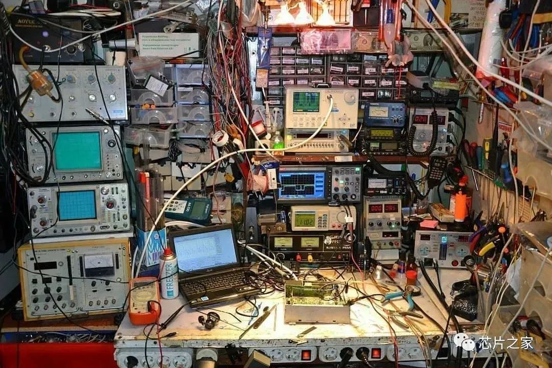
When talking about oscilloscopes, one cannot help but recall the time spent testing at Samsung.The first version of the product’s PCB was followed by time spent in the lab, racing against product cycles, with continuous validation and testing during that period.It has been a long time since I last tested; I feel a bit nostalgic about those devices… Let’s stop there!Back to the point, let’s jump straight to the mind map: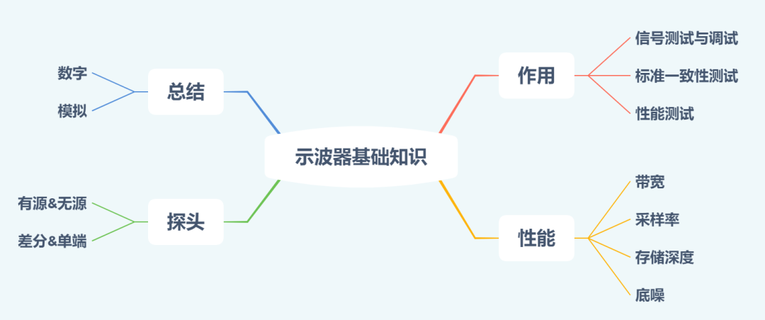
01
Function
When discussing oscilloscopes, the first question that comes to mind is: what is the use of an oscilloscope? Some might answer without hesitation: to measure waveforms. This answer is correct but too vague. Signals can be categorized as low-speed or high-speed, and the standards for testing different signals with an oscilloscope vary. From three perspectives:
For ordinary signals, the requirements for the oscilloscope are not high; it is used for testing and debugging, and many acquaintances have one at hand. However, there are still some requirements; at this time, waveform capture is crucial.
For high-speed signals, the requirements for the oscilloscope increase significantly, making it not something an individual can afford. At this point, standard consistency testing of the signal is necessary, and the oscilloscope must focus on bandwidth, noise floor, and other related performance indicators.
In optical communication, which includes radar, optical modules, etc., the focus is more on the accuracy and trigger bandwidth of the oscilloscope. I have not worked in this area, but I hope to learn more about it in the future.
02
Performance
In the performance section, I will choose four indicators to explain: bandwidth, sampling rate, memory depth, dead time, and noise floor.
Bandwidth
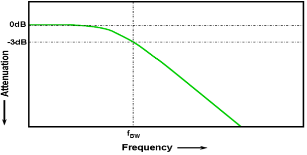
The standard definition: the minimum frequency at which the input signal is attenuated by 3 dB is considered the bandwidth of the oscilloscope. It determines the oscilloscope’s ability to measure high-frequency signals. For example, how do you verify a 1GHz bandwidth oscilloscope? Input a standard 50MHz, 1V peak-to-peak sine wave signal, and measure the signal amplitude as A on the oscilloscope. Keep the input signal amplitude constant and gradually increase the input signal frequency to 1GHz, at which point the measured signal amplitude on the oscilloscope is B. The result of 20lg(B/A) is compared to the -3 dB standard.
To emphasize again, the -3dB here is calculated based on signal power, which corresponds to the signal power being halved. The oscilloscope measures voltage signals, and when the power is halved, according to the relationship, the voltage value measured by the oscilloscope drops to 0.707 times the original.
When it comes to bandwidth, the first thing that comes to my mind is rise time. Do you remember that formula? It’s the one with 0.35. Since the oscilloscope also has a Gaussian frequency response, it conforms to this relationship; the question is how to test it.
We won’t discuss flat response or accuracy here. Of course, we see various formulas on many networks.
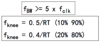
The relationship between bandwidth and clock frequency. The 5 times here requires attention; the premise is that the rise edge is assumed to be 7% of the period. In the formula for the corner frequency, RT is 1/10 of the period.
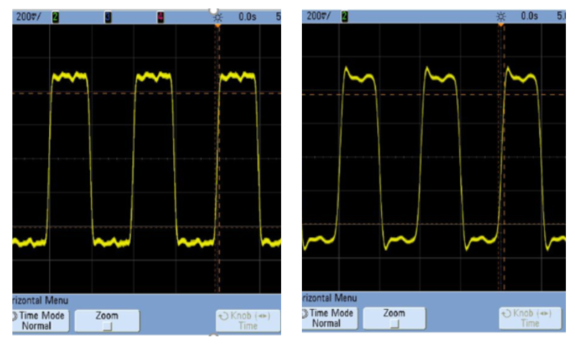
Not to get bogged down in these details, normally, choosing 5 times is sufficient; for example, if the signal to be tested is 100M, the oscilloscope bandwidth should be 500M. If someone wants to know what happens if the selected oscilloscope bandwidth is insufficient, let me show you the difference in measuring different rise time signals with the same bandwidth oscilloscope.
Sampling Rate
After discussing bandwidth, let’s talk about sampling rate. These two major indicators are prominently displayed on the oscilloscope.
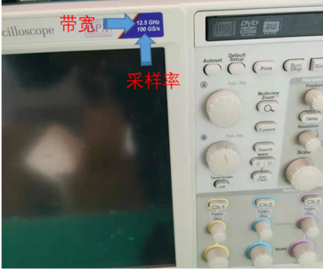
Typically, the sampling rate is four times or higher than the bandwidth, and it is important to note that the oscilloscope operates in a high-frequency response manner.
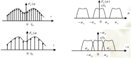
The oscilloscope’s sampling rate is the number of sample points it can acquire per second. When discussing signal sampling, everyone thinks of the Nyquist sampling theorem, which states that the sampling rate must be greater than twice the signal bandwidth to allow the oscilloscope to reconstruct the signal without aliasing.
Memory Depth
When testing signals, we certainly hope to display more information continuously on the screen. The oscilloscope digitizes the input signal through an ADC, and the data of these sampled points is stored in the oscilloscope’s memory. The memory depth is related to the sampling rate and the duration of the screen display. The relevant formula is: sampling rate = memory depth / screen display time.
This indicates that increasing the display time will reduce the sampling rate. Only if the oscilloscope has sufficient memory depth can it collect longer waveforms at high sampling rates.
Dead Time
Digital oscilloscopes differ from analog oscilloscopes in that they cannot process related data in real-time. Digital oscilloscopes collect signals in a non-continuous process, and the time between repeated collections is needed to process and display some collected waveforms. This time is known as dead time. In other words, during this time, the oscilloscope cannot capture signals or display new waveforms. If an abnormal signal occurs during this time, it can lead to information loss, which is detrimental to signal debugging.
It is important to note that dead time is not fixed; it depends on the time taken by the oscilloscope to process data.
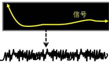
Noise Floor
The noise floor of the oscilloscope is generated by the oscilloscope’s attenuator, front-end amplifier, and A/D converter, which superimposes on the signal and merges with it. In other words, after sampling, the oscilloscope will amplify the signal again, and the noise floor will also be amplified simultaneously.
03
Probes
When testing signals, in addition to focusing on the oscilloscope’s bandwidth, one must also pay attention to the probe bandwidth. If the oscilloscope bandwidth is 1GHz and the probe bandwidth is 500MHz, then the combined system bandwidth is 500MHz. When purchasing an oscilloscope, it generally comes with matching probes.
Probes can be classified into passive probes and active probes.
Passive probes are generally used for low-bandwidth oscilloscopes, with a low bandwidth experience value of 500 MHz, featuring a 10:1 attenuation ratio and high-impedance input, which brings significant capacitive loading. Common power ripple testing probes are passive.
Active probes, as the name suggests, have internal power devices and an internal power amplifier embedded close to the probe body, which can provide lower capacitive loading.
In addition to the classification of passive and active, probes can also be divided into: single-ended probes and differential probes.
Single-ended probes can be either active or passive, while differential probes are generally active probes.
Differential probes have two input terminals, one positive and one negative, along with a separate ground line. The output signal is proportional to the voltage difference between the two input terminals. Differential probes reference each other rather than ground voltage, which distinguishes them from single-ended probes.
The effective grounding between the signal connections in differential probes is more ideal than most grounding layers in single-ended probes. This grounding effectively connects the probe ground line to the device under test (DUT) with very low impedance.
There are also differences in voltage measurement ranges; active probes can only measure a few volts, while passive probes, with high-impedance input, can measure voltages up to several hundred volts.
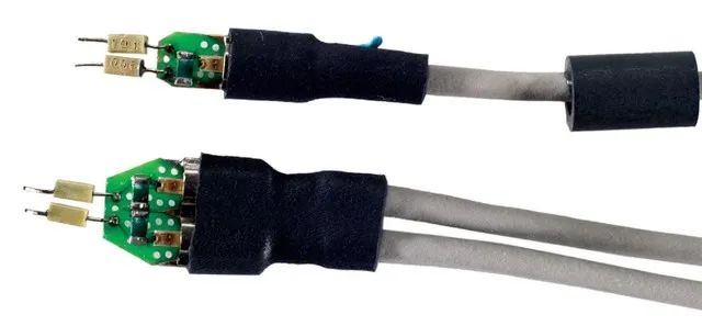
There are also current probes and similar devices, but I have not used them, so I won’t elaborate.
04
Conclusion
Oscilloscopes can be divided into analog and digital types; here we mainly discuss digital oscilloscopes. The signal enters, is sampled by an ADC (analog-to-digital converter), and the sampled digital points are buffered. After internal signal processing, it is converted back to analog by a DAC (digital-to-analog converter) and finally displayed on the screen. Many products operate on this principle, such as the ultrasound devices I worked on previously.
Recommended Reading:
-
Techniques for Drawing Circuit Diagrams
-
Insights on Circuit Diagram Recognition and Analysis Methods
-
A Practical Discussion on MOSFETs
Follow our public account for daily knowledge updates!
👇