


As we all know, MATLAB is not only good at handling numerical calculations related to matrices, but it also has a deep foundation in scientific visualization. The numerous rich functions it provides can well meet our various needs for using graphics to display numerical information.
MATLAB has the ability to represent graphics in two-dimensional, three-dimensional, and even four-dimensional forms. It can express data characteristics from aspects such as line type, boundary color, color, rendering, lighting, and perspective.
The visualization capabilities of MATLAB are based on a set of graphics objects. The core of graphics objects is the operation of the graphics handle (Graphics Handle).
Some commonly used low-level commands are as follows:
gcf: Returns the handle of the current window object (Get Current Figure)
gca: Returns the handle of the current axis object (Get Current Axes)
gco: Returns the handle of the current graphic object (Get Current Object)
get: Obtains the properties of the handle graphic object and returns certain object handle values
set: Changes the properties of the graphic object
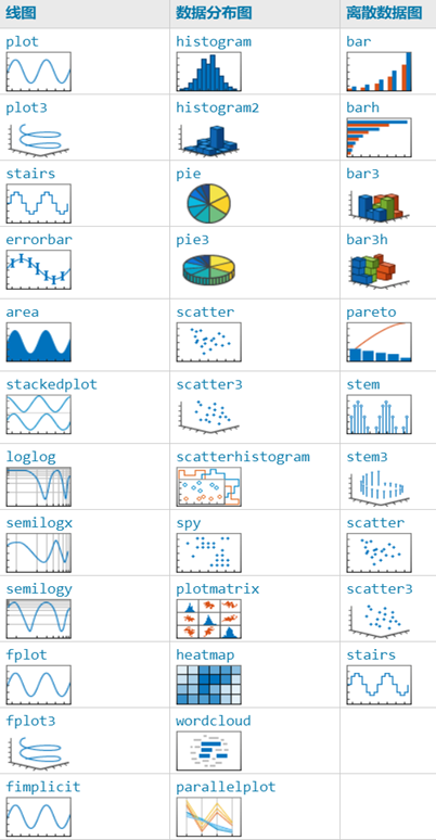
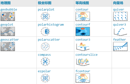
This article mainly introduces some high-level plotting commands and related functions:
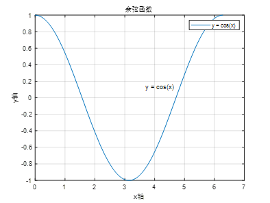
x=0:0.01:2*pi;
y=cos(x);
plot(x,y);
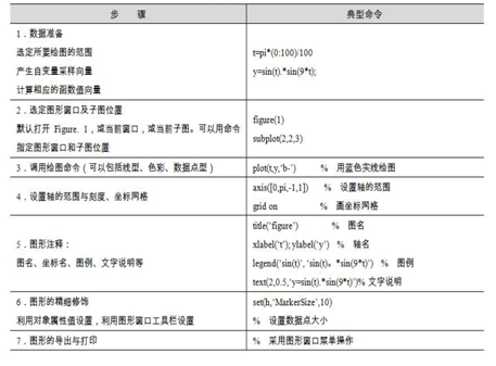
xlabel(‘x-axis’); % x-axis annotation
ylabel(‘y-axis’); % y-axis annotation
title(‘Cosine Function’); % Graph title
legend(‘y = cos(x)’); % Graph annotation
gtext(‘y = cos(x)’); % Graph annotation, use mouse to position the annotation
grid on; % Show grid lines
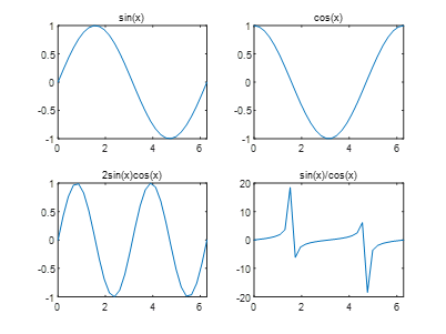
Establish several coordinate systems on the same screen using the subplot(m,n,p) command;
Divide a screen into m×n graphic areas, where p represents the current area number, and draw a graph in each area.
x=linspace(0,2*pi,30);y=sin(x); z=cos(x);
u=2*sin(x).*cos(x);v=sin(x)./cos(x);
subplot(2,2,1),plot(x,y),axis([0 2*pi -1 1]),title(‘sin(x)’)
subplot(2,2,2),plot(x,z),axis([0 2*pi -1 1]),title(‘cos(x)’)
subplot(2,2,3),plot(x,u),axis([0 2*pi -1 1]),title(‘2sin(x)cos(x)’)
subplot(2,2,4),plot(x,v),axis([0 2*pi -20 20]),title(‘sin(x)/cos(x)’)
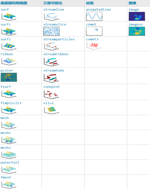
When plotting three-dimensional graphs in MATLAB, the most commonly used functions are surf, mesh, and their derivative functions.
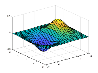
x=linspace(-2,2, 25); % Take 25 points on the x-axis y=linspace(-2, 2, 25); % Take 25 points on the y-axis [xx,yy]=meshgrid(x, y); % xx and yy are both 21×21 matrices zz=xx.*exp(-xx.^2-yy.^2); % Calculate function values, zz is also a 21×21 matrix surf(xx, yy, zz); % Plot the surface graph
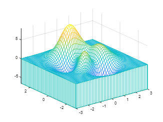
Using the peaks function as an example, plot in various ways with the same colormap 1. meshz can add a skirt to the surface: [x,y,z]=peaks;meshz(x,y,z);axis([-inf inf -inf inf -inf inf]);
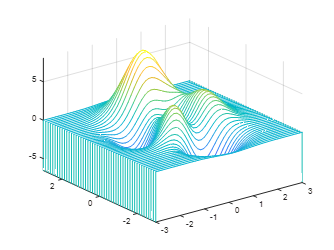
2. waterfall can create a water flow effect in the x direction or y direction:[x,y,z]=peaks;waterfall(x,y,z);axis([-inf inf -inf inf -inf inf]);
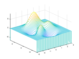
3. Water flow effect in the y direction:[x,y,z]=peaks;waterfall(x’,y’,z’);axis([-inf inf -inf inf -inf inf]);
4. meshc can simultaneously draw a mesh graph and contour lines:[x,y,z]=peaks;meshc(x,y,z);axis([-inf inf -inf inf -inf inf]);
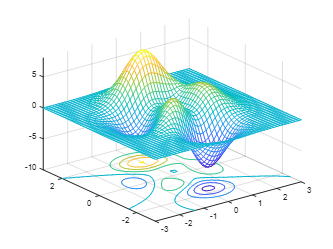
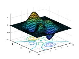
5. surfc can simultaneously draw a surface graph and contour lines:[x,y,z]=peaks;surfc(x,y,z);axis([-inf inf -inf inf -inf inf]);
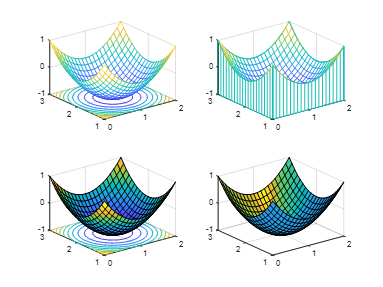
6. Compare the four functions meshc, meshz, surfc, surfl
[x,y]=meshgrid(0:0.1:2,1:0.1:3)
z=(x-1).^2+(y-2).^2-1
subplot(2,2,1);meshc(x,y,z)
subplot(2,2,2);meshz(x,y,z)
subplot(2,2,3);surfc(x,y,z)
subplot(2,2,4);surfl(x,y,z)
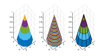
For example, using the same colormap, plot a cone in different coloring methods.
[x,y,z] =cylinder(pi:-pi/5:0,10)
colormap(lines)
subplot(1,3,1)
surf(x,y,z);
shading flat
subplot(1,3,2)
surf(x,y,z);
shading interp
subplot(1,3,3)
surf(x,y,z)
Author: Senior Zhang from Extreme Value Academy

Click to Read the Original Text
Register Now to Participate