MATLAB – Simple Implementation of Numerical PDE Solving
Introduction
Traditional numerical methods for solving PDEs include characteristic line methods, finite element methods, boundary element methods, multigrid methods, spectral methods, Fourier transform methods, etc. Due to limitations in knowledge, this article will only utilize Finite Difference, FT, and Characteristic Line Methods to implement numerical solutions for PDEs in MATLAB.
Table of Contents
-
1. Heat Conduction Equation (Finite Difference Method) -
2. Wave Equation (Finite Difference Method) -
3. Heat Conduction Equation (Fourier Transform) -
4. Heat Conduction in a Plate (Explicit Difference Method) -
5. Wave Equation (Characteristic Line Method)
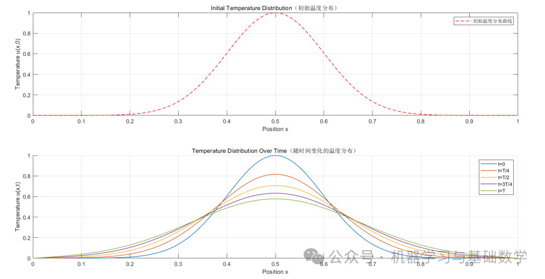
1. Heat Conduction Equation (Finite Difference Method)
Finite Difference Method:
Transforming the continuous PDE into a discrete form, the finite difference method approximates derivatives to obtain numerical solutions. Common variants include explicit and implicit methods, as well as the Crank-Nicolson method.
Using a rectangular grid covering the plane with directional step sizes, for numerical simulation, the backward difference scheme is utilized:
This scheme satisfies the Courant-Friedrichs-Lewy criterion, and the solution of the backward difference scheme converges to the solution of the partial differential equation.
1.1 MATLAB Code
%% Heat Conduction Equation 2d&3d
% Parameter settings
L = 1; % Length of the region
Nx = 100; % Number of spatial points
dx = L / Nx; % Spatial step size
x = (0:Nx) * dx; % Spatial grid
T = 1.0; % Total time
Nt = 1000; % Number of time steps
dt = T / Nt; % Time step size
alpha = 0.01; % Thermal diffusion coefficient
% Initial condition follows Gaussian distribution
sigma = 0.1;
u0 = exp(-(x - 0.5*L).^2 / (2*sigma^2));
% Preallocate temperature matrix
u = zeros(Nx+1, Nt+1);
u(:, 1) = u0';
% Numerical solution using Forward Time Centered Space (FTCS)
for n = 1:Nt
for i = 2:Nx
u(i, n+1) = u(i, n) + alpha * dt / dx^2 * (u(i+1, n) - 2*u(i, n) + u(i-1, n));
end
end
% Plotting
figure;
subplot(2,1,1);
plot(x, u(:, 1), 'r--', 'LineWidth', 1);
xlabel('Position x');
ylabel('Temperature u(x,0)');
title('Initial Temperature Distribution');
legend('Initial Temperature Distribution Curve');
grid on;
subplot(2,1,2);
hold on;
for n = 1:floor(Nt/4):Nt+1
plot(x, u(:, n), 'LineWidth', 1);
end
hold off;
xlabel('Position x');
ylabel('Temperature u(x,t)');
title('Temperature Distribution Over Time');
grid on;
legend('t=0', 't=T/4', 't=T/2', 't=3T/4', 't=T');
% Extract initial and final temperature distributions
u_initial = u(:, 1);
u_final = u(:, end);
[X, T] = meshgrid(x, linspace(0, T, Nt+1)); % Adjust T to match time steps
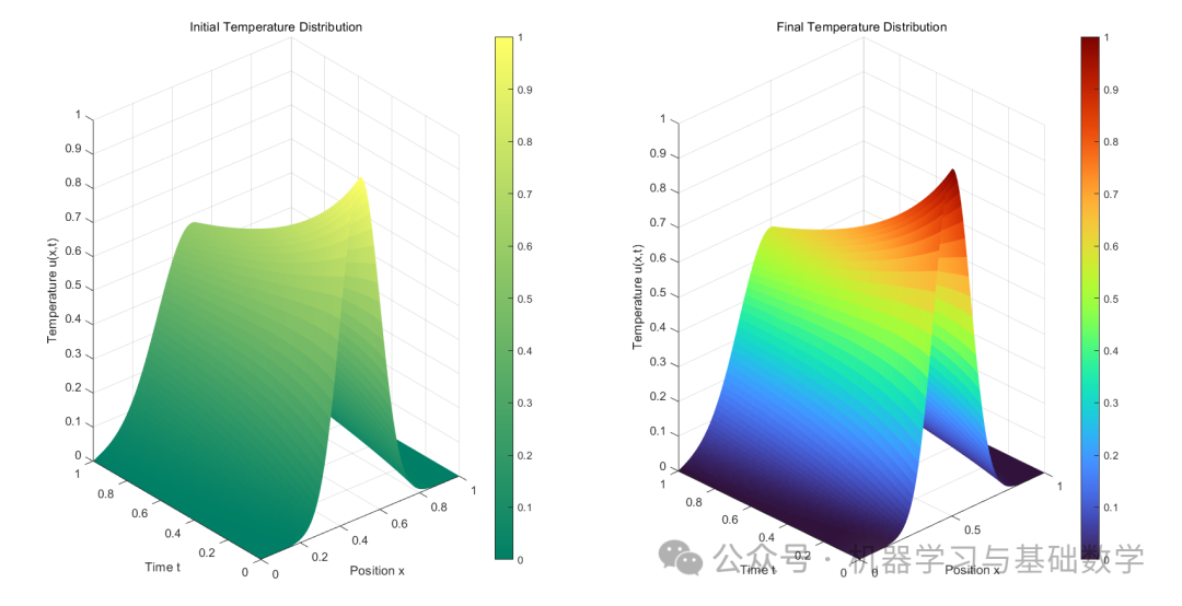
% Draw initial temperature distribution plot
figure;
subplot(1, 2, 1);
surf(X, T, u(:, 1:Nt+1)', 'EdgeColor', 'none');
xlabel('Position x');
ylabel('Time t');
zlabel('Temperature u(x,t)');
title('Initial Temperature Distribution');
view(3);
grid on;
colorbar;
% Draw final temperature distribution plot
subplot(1, 2, 2);
surf(X, T, u(:, 1:Nt+1)', 'EdgeColor', 'none');
xlabel('Position x');
ylabel('Time t');
zlabel('Temperature u(x,t)');
title('Final Temperature Distribution');
view(3);
grid on;
colorbar;
1.2 Plotting
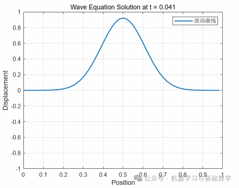
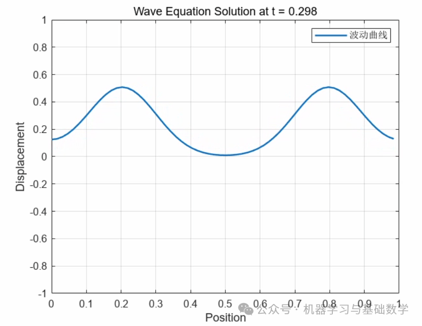
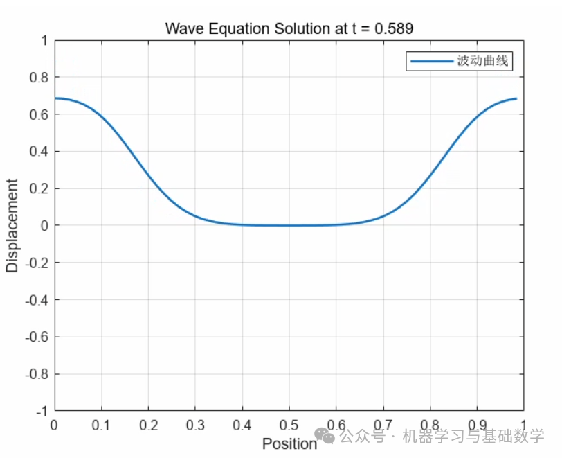
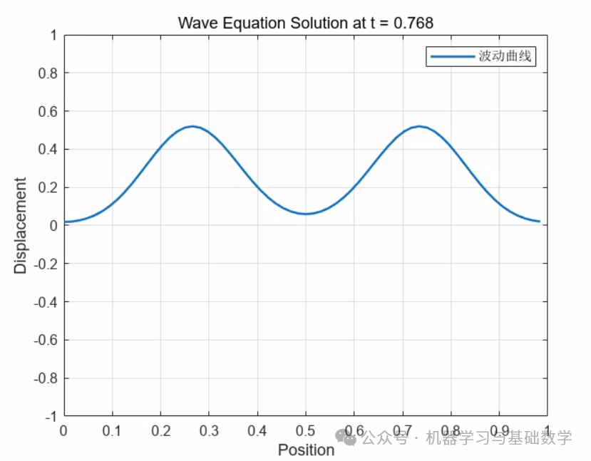
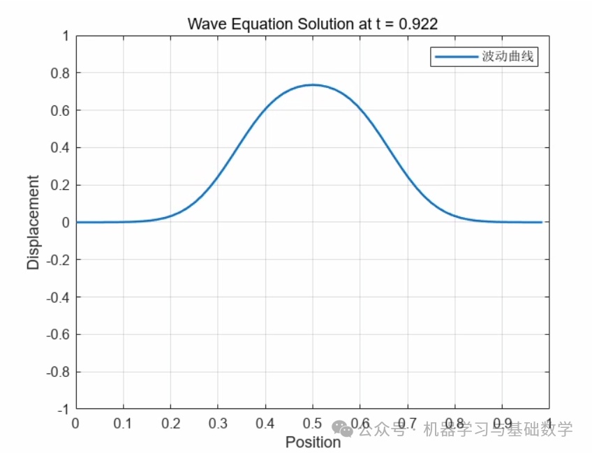
2. Wave Equation (Finite Difference Method)
2.1 MATLAB Code
L = 1;
Nx = 64;
x = linspace(0, L, Nx+1);
x = x(1:Nx);
dx = x(2) - x(1);
Nt = 1000;
t_final = 1.0;
dt = t_final / Nt;
% Initial conditions
u0 = exp(-((x - 0.5*L).^2) / (2*0.1^2));
v0 = zeros(1, Nx);
% Initialize velocity (v) and displacement (u)
u = zeros(Nx, Nt+1);
v = zeros(Nx, Nt+1);
u(:, 1) = u0';
v(:, 1) = v0';
% Time integration loop (using finite difference)
for n = 1:Nt
u_new = u(:, n) + dt * v(:, n);
v_new = v(:, n) + dt * (1/dx^2) * (circshift(u(:, n), -1) - 2*u(:, n) + circshift(u(:, n), 1));
u(:, n+1) = u_new;
v(:, n+1) = v_new;
end
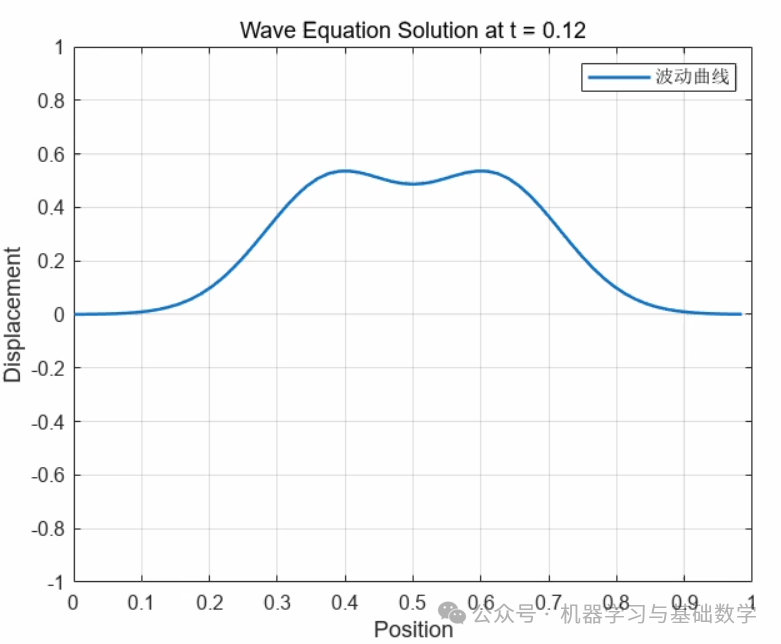
figure;
for n = 1:Nt+1
plot(x, u(:, n), 'LineWidth', 1.5);
grid on
legend("Wave Curve")
xlabel('Position');
ylabel('Displacement');
title(['Wave Equation Solution at t = ' num2str((n-1)*dt)]);
ylim([-1 1]);
pause(0.01);
end
2.2 Plotting
1. t=0.041
2. t=0.12
3. t=0.298
4. t=0.589
5. t=0.768
6. t=0.922
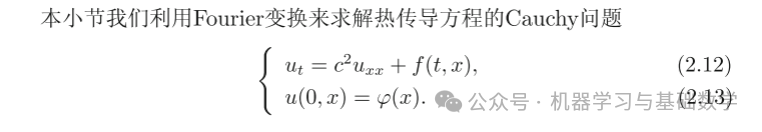
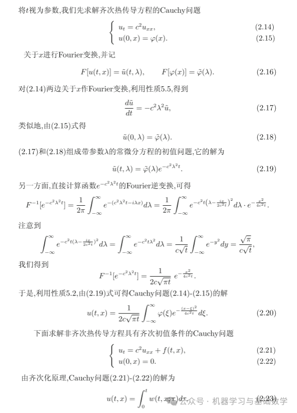
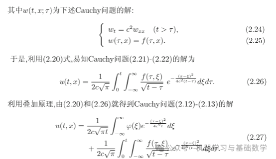
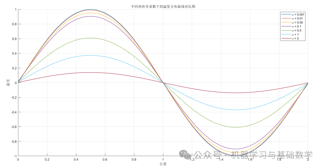
3. Heat Conduction Equation (Fourier Transform)
Introducing Fourier transform within the scope of generalized functions imposes almost no restrictions from other conditions, making the Fourier transform more flexible in PDEs.
Mathematical Derivation of Fourier Transform:
Fourier Transform:
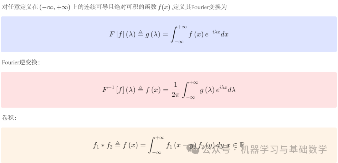
Several Properties of Fourier Transform:

3.1 MATLAB Code
L = 2; % Length of the solving region
N = 200; % Number of discrete grids
dx = L / N; % Grid spacing
x = linspace(0, L, N); % Grid points
u0 = sin(pi*x); % Initial temperature distribution, e.g., sine function
timesteps = 100; % Number of time steps
dt = 0.001; % Time step size
% Different thermal diffusion coefficients
alphas = [0.001, 0.01, 0.05, 0.1, 0.5, 1, 2];
% Initialize array to store results
results = zeros(length(alphas), N);
% Loop to calculate results for each thermal diffusion coefficient
for i = 1:length(alphas)
alpha = alphas(i);
k = fftshift((2*pi/L)*(-N/2:N/2-1)); % Fourier frequency vector
u = fft(u0); % Perform Fourier transform on the initial temperature field
for n = 1:timesteps
u = u .* exp(-alpha*(k.^2)*dt); % Solution in the frequency domain
end
u = ifft(u); % Convert the transformed results back to the spatial domain
results(i, :) = real(u); % Store results
end
% Visualization of results
figure;
hold on;
for i = 1:length(alphas)
plot(x, results(i, :), 'LineWidth', 1, 'DisplayName', ['\alpha = ', num2str(alphas(i))]);
end
hold off;
xlabel('Position');
ylabel('Temperature');
title('Comparison of Temperature Distribution Curves under Different Thermal Diffusion Coefficients');
legend show;
grid on;
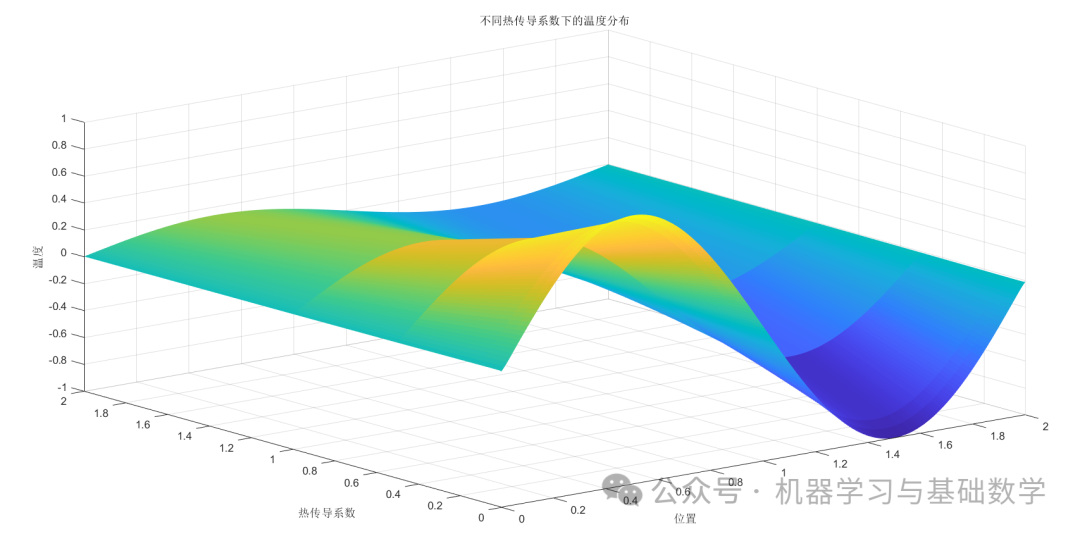
% 3D Visualization
figure;
[X, Y] = meshgrid(x, alphas);
surf(X, Y, results, 'EdgeColor', 'none');
xlabel('Position');
ylabel('Thermal Diffusion Coefficient');
zlabel('Temperature');
title('Temperature Distribution under Different Thermal Diffusion Coefficients');
3.2 Plotting
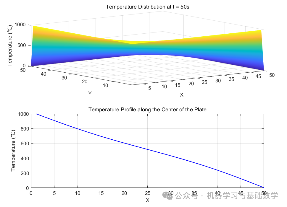
4. Heat Conduction in a Plate (Explicit Difference Method)
A small experiment from the past (hihi~~)
4.1 MATLAB Code
%% Iron Plate Heat Conduction Curve and Animation
% Set parameters for the iron plate
Lx = 0.1; % Length of the iron plate (m)
Ly = 0.1; % Width of the iron plate (m)
Nx = 50; % Number of discrete points (x direction)
Ny = 50; % Number of discrete points (y direction)
dx = Lx / (Nx - 1); % Discrete step (x direction)
dy = Ly / (Ny - 1); % Discrete step (y direction)
alpha = 1e-4; % Thermal diffusion coefficient (m^2/s)
T0 = 1000; % Initial temperature of the iron plate (℃)
T_air = 2; % External ambient temperature (℃)
dt = 0.01; % Time step (s)
t_max = 50; % Maximum simulation time (s)

% Initialize temperature field
T = T0 * ones(Nx, Ny);

% Create figure window
figure;

% Create first subplot for displaying 3D temperature change graph
subplot(2,1,1);
surf(T);
xlabel('X');
ylabel('Y');
zlabel('Temperature (℃)');
title('Temperature Distribution');
axis([1 Nx 1 Ny 0 T0]);
shading interp;
view(3);

% Create second subplot for displaying temperature curve along the center of the plate
subplot(2,1,2);
h = plot(T(:, round(Ny/2)), 'LineWidth', 1.2,'Color',[0 0 1]);
xlabel('X');
ylabel('Temperature (℃)');
title('Temperature Profile along the Center of the Plate');
grid on;

% Perform heat conduction simulation
for t = 1:round(t_max/dt)
    T_new = T;
    for i = 2:Nx-1
        for j = 2:Ny-1
            % Calculate temperature for the next time step using explicit difference method
            T_new(i,j) = T(i,j) + alpha * dt * ((T(i+1,j) - 2*T(i,j) + T(i-1,j)) / dx^2 + (T(i,j+1) - 2*T(i,j) + T(i,j-1)) / dy^2);
        end
    end
    T = T_new;

    % Boundary conditions: temperature at the edges of the iron plate remains unchanged
    T(1,:) = T0;
    T(Nx,:) = T0;
    T(:,1) = T0;
    T(:,Ny) = T0;

    % Boundary conditions: ambient temperature
    T(Nx,:) = T_air;
    T(:,Ny) = T_air;

    % Update temperature curve
    set(h, 'YData', T(:, round(Ny/2)));

    % Update 3D temperature change graph
    if mod(t, 100) == 0
        subplot(2,1,1);
surf(T);
        xlabel('X');
ylabel('Y');
zlabel('Temperature (℃)');
title(['Temperature Distribution at t = ', num2str(t*dt), 's']);
        axis([1 Nx 1 Ny 0 T0]);
        shading interp;
        view(3);
    end

    drawnow;
end
4.2 Plotting
5. Wave Equation (Characteristic Line Method)
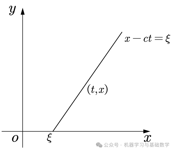
Method of Characteristics:
Applicable to unconventional forms of PDEs, such as convection-diffusion equations, solving through the direction of characteristic lines.
In the plane, define a family of characteristic lines along any straight line of the family of characteristic curves:
The equation satisfies
Thus, along such a straight line, remains constant, it only relates to the parameters of different lines in the family of characteristics.
Therefore, the equation has a general solution form:
The above indicates that the general solution is uniquely determined by initial values.
5.1 MATLAB Code
%% Characteristic Line Method to Solve Wave Equation
% Parameter settings
L = 10; % Spatial length
T = 5; % Total time
c = 1.5; % Wave speed
dx = 0.1; % Spatial step size
dt = 0.01; % Time step size
% Discretize space and time
x = 0:dx:L; % Spatial grid
t = 0:dt:T; % Time grid
% Initialize wave function u(x, t)
u = zeros(length(x), length(t));
% Initial and boundary conditions
u(:,1) = sin(pi*x/L); % Initial wave shape, assumed to be a sine wave
u(1,:) = 0; % Left boundary condition
u(end,:) = 0; % Right boundary condition
% Solve wave equation using the method of characteristics
for n = 1:length(t)-1
for i = 2:length(x)-1
u(i,n+1) = u(i,n) + dt*c/dx * (u(i+1,n) - u(i,n)); % Update wave function value using the method of characteristics
end
end
% Visualize the evolution of the wave equation
[X, T] = meshgrid(t, x);
figure;
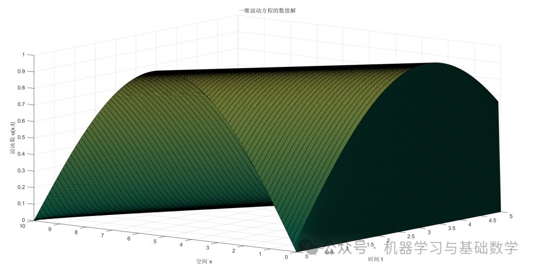
surf(X, T, u);
xlabel('Time t');
ylabel('Space x');
zlabel('Wave Function u(x,t)');
title('Numerical Solution of One-Dimensional Wave Equation');
5.2 Plotting
 Follow the public account [Machine Learning and Basic Mathematics] to get knowledge nuggets without getting lost!
The Klein bottle is a non-orientable two-dimensional compact manifold, while the sphere or torus is an orientable two-dimensional compact manifold. If we observe the Klein bottle, one point seems puzzling – the neck and body of the Klein bottle intersect, in other words, some points on the neck and some points on the wall occupy the same position in three-dimensional space. We can understand the Klein bottle in four-dimensional space: the Klein bottle is a surface that can only be truly represented in four-dimensional space. If we really have to represent it in our three-dimensional space, we have to compromise a bit and represent it as if it intersects with itself. The neck of the Klein bottle passes through the fourth-dimensional space and connects to the base ring, without passing through the wall. To use a knot as a metaphor, if we regard it as a curve on a plane, it seems to intersect with itself, but upon closer inspection, it seems to break into three sections. However, it is easy to understand that this shape is actually a curve in three-dimensional space. It cannot intersect with itself in a plane, but if there is a third dimension, it can pass through the third dimension to avoid intersecting with itself. It is the same with the Klein bottle; we can understand it as a surface in four-dimensional space. In our three-dimensional space, even the most skilled craftsman has to make it appear as if it intersects with itself; just as the most skilled painter, when drawing a knot on paper, must also draw it as if it intersects with itself. Interestingly, if we cut the Klein bottle along its axis of symmetry, we will get two Möbius strips. If the Möbius strip can perfectly showcase a “one-dimensional model of infinitely extendable space in two-dimensional space,” the Klein bottle can only serve as a reference for exhibiting a “two-dimensional model of infinitely extendable space in three-dimensional space.” Because in the process of making the Möbius strip, we have to twist the paper strip 180° and then join the ends, this is an operation under three-dimensional space. The ideal “two-dimensional model of infinitely extendable space in three-dimensional space” should be a model where moving in any direction on the two-dimensional surface can return to the origin, whereas the Klein bottle, although it can infinitely progress in any direction on the two-dimensional surface, can only return to the origin in two specific directions, and only in one direction will it pass through a “reverse origin” before returning to the origin. The truly ideal “two-dimensional model of infinitely extendable space in three-dimensional space” should also be one that passes through a “reverse origin” once before returning to the origin when moving in any direction on the two-dimensional surface. Making this model requires distorting the three-dimensional model in four-dimensional space. An important branch of mathematics is called topology, which mainly studies the characteristics and laws of geometric figures when their shapes change continuously. The Klein bottle and the Möbius strip have become one of the most interesting problems in topology. The concept of the Möbius strip is widely applied in architecture, art, and industrial production. The three-dimensional Klein bottle is defined in topology as a square region [0,1]×[0,1] with equivalence relations (0,y)~(1,y), 0≤y≤1 and (x,0)~(1-x,1), 0≤x≤1. Similar to the Möbius strip, the Klein bottle is non-orientable. However, the Möbius strip can be embedded in three-dimensional space, while the Klein bottle can only be embedded in four-dimensional (or higher-dimensional) space. The Möbius strip is created by taking a strip of paper, twisting one section 180°, and then gluing the two ends together. This is also a surface with only one side, but unlike the sphere, torus, and Klein bottle, it has an edge (note that it only has one edge). If we glue two Möbius strips along their only edge, we will get a Klein bottle (of course, we must not forget that we can only truly complete this gluing in four-dimensional space, otherwise, we would have to tear the paper a little). Similarly, if we cut a Klein bottle appropriately, we can obtain two Möbius strips. In addition to the shape of the Klein bottle we have seen above, there is also a lesser-known “8-shaped” Klein bottle. It looks completely different from the surface above, but in four-dimensional space, they are actually the same surface – the Klein bottle. In fact, it can be said that the Klein bottle is a 3° Möbius strip. We know that if we draw a circle on a plane and put something inside it, if we take it out in two-dimensional space, we must cross the circle’s boundary. However, in three-dimensional space, it is easy to take it out without crossing the boundary. The trajectory of the object along with the original circle projected into two-dimensional space is a “two-dimensional Klein bottle,” which is the Möbius strip (the Möbius strip here refers to the topological meaning of the Möbius strip). Now imagine that in our three-dimensional space, it is impossible to take the yolk out of an egg without breaking the shell, but in four-dimensional space, it can be done. The trajectory of the yolk along with the shell projected into three-dimensional space must show a Klein bottle. Historical experiences show that the German mathematician Klein once proposed the “impossible” hypothesis, that is, the topological monster – the Klein bottle. This bottle has no inside or outside, no matter where you penetrate the surface, you still arrive outside the bottle, so it is essentially a strange thing with “outside but no inside.” Although modern glass manufacturing has developed very advanced, the so-called “Klein bottle” has always been a “fictional object” in the mind of the great mathematician Klein, which can never be manufactured. Mathematicians from many countries have been trying to create one as a gift for the International Mathematical Congress. However, what awaits them is one failure after another. Some also believe that even if they cannot create a glass product, making a paper model would be great. If they really solve this problem, it would be a significant achievement!