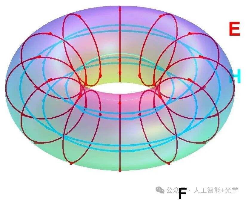
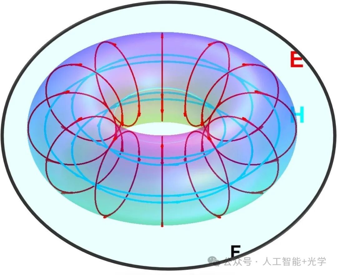
 IntroductionFollowing our previous article where we plotted scalar topological vortex surfaces, this time we will learn how to plot vector field surfaces, as physical fields are often vector fields. Let’s dive straight into the content!
🌄 MATLAB Vector Topological Vortex Surface Plot
    clc     clear all    close all    %% Vector Topological Vortex    % Initialize window    figure('Color', 'w', 'Position', [100, 100, 800, 600]);    hold on;    axis equal;    axis off;
    %% Parameter Settings    R = 4; % Major Radius - Distance from the center of the torus to the center of the pipe    r = 1.5; % Minor Radius - Radius of the pipe
    %% 1. Draw the orange toroidal surface (Surface)    % Generate mesh data    [theta, phi] = meshgrid(linspace(0, 2*pi, 100), linspace(0, 2*pi, 50));
    % Toroidal parameter equations    X = (R + r * cos(phi)) .* cos(theta);    Y = (R + r * cos(phi)) .* sin(theta);    Z = r * sin(phi);
    % Draw surface    hSurf = surf(X, Y, Z);
    % Set material and lighting effects    set(hSurf, 'FaceColor', [1, 0.6, 0.1], ... % Orange               'EdgeColor', 'none', ...      % Remove grid lines               'FaceAlpha', 0.8, ...         % Set transparency               'AmbientStrength', 0.4, ...               'DiffuseStrength', 0.6, ...               'SpecularStrength', 0.5);
    %% 2. & 3. Draw red streamlines and arrows     num_rings = 12; % Number of red rings    ring_angles = linspace(0, 2*pi, num_rings + 1);     ring_angles(end) = []; % Remove the last duplicate angle
    % For generating a single streamline's phi angle    t = linspace(0, 2*pi, 100);
    for i = 1:num_rings        th = ring_angles(i); % Fixed angle of the current ring on the large circle
        % Calculate streamline coordinates (poloidal wrapping)        % Note: In the figure, the lines wrap around the pipe (Poloidal direction)        x_line = (R + (r + 0.05) * cos(t)) * cos(th); % r+0.05 is to slightly lift the line above the surface        y_line = (R + (r + 0.05) * cos(t)) * sin(th);        z_line = (r + 0.05) * sin(t);
        % Draw lines        plot3(x_line, y_line, z_line, 'r-', 'LineWidth', 2);
        % --- Add arrows ---        % Select several points on each line to draw arrows        arrow_indices = 10:25:90; % Select several positions on the line
        for idx = arrow_indices            % Current point coordinates            p0 = [x_line(idx), y_line(idx), z_line(idx)];
            % Calculate tangent vector (derivative)            % dx/dt = -r*sin(t)*cos(th)            % dy/dt = -r*sin(t)*sin(th)            % dz/dt = r*cos(t)
            dt_val = t(idx);            vx = -(r) * sin(dt_val) * cos(th);            vy = -(r) * sin(dt_val) * sin(th);            vz = (r) * cos(dt_val);
            % Normalize vector and scale            vec = [vx, vy, vz];            vec = vec / norm(vec) * 0.8; % Length 0.8
            % Use quiver3 to draw arrows            q = quiver3(p0(1), p0(2), p0(3), vec(1), vec(2), vec(3), 0);
            % Set arrow style            set(q, 'Color', 'r', 'LineWidth', 2, 'MaxHeadSize', 0.5, 'ShowArrowHead', 'on');        end    end
    %% 4. Beautify the environment    % Add lighting    light('Position', [10, 10, 10], 'Style', 'local');    light('Position', [-10, -10, 10], 'Style', 'local');    lighting gouraud; % Smooth lighting
    % Adjust title    title('Vector Toroidal Vortex', 'FontSize', 16, 'FontName', 'Arial');
    % Rotate the view slightly to match the 3D effect of the image    view(45, 45);
    hold off;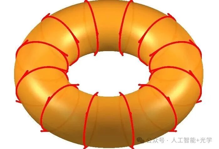
% Initialize window figure('Color', 'w', 'Position', [100, 100, 800, 700]); hold on; axis equal; axis off;
% Set view angle (match the perspective angle of the original image) view(-30, 35);
%% Core Parameters R = 4; % Major Radius (Distance from the center of the ring to the center of the pipe) r_shell = 2.0; % Shell Radius (widest) r_red = 1.95; % Red line radius (close to the surface) r_blue = 1.2; % Blue line radius (located in the inner core)
%% 1. Draw semi-transparent rainbow shell (Scalar Shell) % Generate mesh num_pts = 120; [theta, phi] = meshgrid(linspace(0, 2*pi, num_pts), linspace(0, 2*pi, num_pts));
% Toroidal coordinates X = (R + r_shell .* cos(phi)) .* cos(theta); Y = (R + r_shell .* cos(phi)) .* sin(theta); Z = r_shell .* sin(phi);
% Color mapping (changes based on the poloidal angle phi) % Adjust phase_shift to make the outer side appear yellow-green and the inner side appear purple-red phase_shift = 3.5; C = mod(phi + phase_shift, 2*pi);
% Draw surface hSurf = surf(X, Y, Z, C);
% Beautify the shell colormap(hsv); % Rainbow color map shading interp; % Smooth interpolation, remove grid lines set(hSurf, 'FaceAlpha', 0.3, ... % Key: set transparency (0.0-1.0) 'EdgeColor', 'none', ... 'AmbientStrength', 0.5, ... 'DiffuseStrength', 0.5, ... 'SpecularStrength', 0.6);
%% 2. Draw red poloidal coils (E Field - Poloidal) % These coils rotate around the cross-section of the pipe
num_red_loops = 12; % Number of coils red_angles = linspace(0, 2*pi, num_red_loops+1); red_angles(end) = [];
t = linspace(0, 2*pi, 100); % Single loop parameters
for th = red_angles % Calculate coordinates of a single red line xr = (R + r_red * cos(t)) * cos(th); yr = (R + r_red * cos(t)) * sin(th); zr = r_red * sin(t);
% Draw lines plot3(xr, yr, zr, 'Color', [0.8, 0, 0], 'LineWidth', 1.5);
% --- Add red arrows --- % Select several points on each line to draw arrows arrow_indices = [20, 50, 80]; % Arrow positions for idx = arrow_indices: p = [xr(idx), yr(idx), zr(idx)];
% Poloidal tangent vector (derivative) vx = -sin(t(idx)) * cos(th); vy = -sin(t(idx)) * sin(th); vz = cos(t(idx));
% Normalize and scale vec = [vx, vy, vz]; vec = vec / norm(vec) * 0.6;
quiver3(p(1), p(2), p(3), vec(1), vec(2), vec(3), 0, ... 'Color', 'r', 'LineWidth', 2, 'MaxHeadSize', 0.8); end end
%% 3. Draw blue toroidal coils (H Field - Toroidal) % These coils rotate along the large circle direction of the torus (located inside the pipe)
% We select several positions inside the pipe to place blue lines (e.g., inner side, outer side, top, bottom) blue_phi_angles = [0, pi/2, pi, 3*pi/2];
t_blue = linspace(0, 2*pi, 200);
for phi_val = blue_phi_angles % Calculate coordinates of a single blue line xb = (R + r_blue * cos(phi_val)) .* cos(t_blue); yb = (R + r_blue * cos(phi_val)) .* sin(t_blue); zb = r_blue * sin(phi_val) .* ones(size(t_blue));
% Draw lines (using Cyan color, clearer against the rainbow background) plot3(xb, yb, zb, 'c-', 'LineWidth', 2);
% --- Add blue arrows --- arrow_indices = 15:30:200; % More arrows for idx = arrow_indices: p = [xb(idx), yb(idx), zb(idx)];
% Toroidal tangent vector (along the large circle tangent) vx = -sin(t_blue(idx)); vy = cos(t_blue(idx)); vz = 0;
vec = [vx, vy, vz]; vec = vec / norm(vec) * 0.6;
quiver3(p(1), p(2), p(3), vec(1), vec(2), vec(3), 0, ... 'Color', 'c', 'LineWidth', 2, 'MaxHeadSize', 0.8); end end
%% 4. Labeling Text (Labels) % Calculate text positions to make them appear to float in the corresponding areas % E (Red) text(R+r_shell+0.5, 0, 1.5, 'E', 'Color', 'r', 'FontSize', 24, ... 'FontWeight', 'bold', 'FontName', 'Arial');
% H (Blue) text(R+r_shell+0.5, 0, -1.5, 'H', 'Color', 'c', 'FontSize', 24, ... 'FontWeight', 'bold', 'FontName', 'Arial');
% F (Title/Bottom label) text(0, -(R+r_shell), -3, 'F', 'Color', 'k', 'FontSize', 20, 'FontWeight', 'bold');
title('Hybrid Toroidal Vortex', 'FontSize', 18);
%% 5. Lighting and Environment Settings % Set lights to enhance the 3D effect and reflections of the transparent material light('Position', [0, -20, 10], 'Style', 'local'); % Front light light('Position', [10, 10, 10], 'Style', 'local'); % Side fill light lighting phong; % Make highlights smoother
% Slightly zoom in camzoom(1.1);
hold off;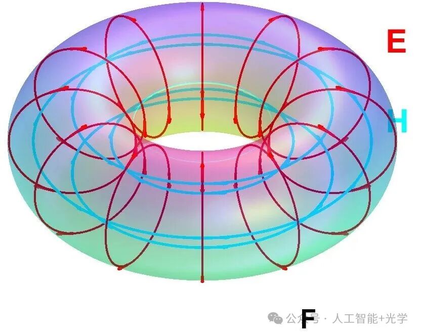 🌄 PythonVector Toroidal Vortex Plotting
import numpy as np
import matplotlib.pyplot as plt
from mpl_toolkits.mplot3d import Axes3D
from matplotlib.colors import LightSource
from matplotlib import cm
# ==========================#  Initialize window# ==========================fig = plt.figure(figsize=(8, 6))
fig.patch.set_facecolor('white')
ax = fig.add_subplot(111, projection='3d')
ax.set_box_aspect((1, 1, 1))  ax.set_axis_off()             # ==========================#  Parameter Settings# ==========================R = 4.0   # Major Radius
r = 1.5   # Minor Radius
# ==========================#  1. Draw the toroidal surface# ==========================theta, phi = np.meshgrid(    np.linspace(0, 2 * np.pi, 100),    np.linspace(0, 2 * np.pi, 50))
X = (R + r * np.cos(phi)) * np.cos(theta)
Y = (R + r * np.cos(phi)) * np.sin(theta)
Z = r * np.sin(phi)
# Use LightSource for simple lighting effect
ls = LightSource(azdeg=45, altdeg=45)
rgb = ls.shade(Z, cmap=cm.Oranges, vert_exag=1, blend_mode='soft')
surf = ax.plot_surface(    X, Y, Z,    facecolors=rgb,           linewidth=0,    antialiased=True,    alpha=0.8,    shade=False           )
# ==========================#  2 & 3. Draw red streamlines and arrows# ==========================num_rings = 12                        ring_angles = np.linspace(0, 2 * np.pi, num_rings + 1)[:-1]
t = np.linspace(0, 2 * np.pi, 100)     for th in ring_angles:    # Poloidal wrapped streamlines, radius slightly larger than r, to make the lines "float" above the surface    x_line = (R + (r + 0.05) * np.cos(t)) * np.cos(th)    y_line = (R + (r + 0.05) * np.cos(t)) * np.sin(th)    z_line = (r + 0.05) * np.sin(t)    ax.plot3D(x_line, y_line, z_line, 'r-', linewidth=2)    # Select several points on the line to draw arrows    arrow_indices = [10, 35, 60, 85]    for idx in arrow_indices:        # Current point coordinates        p0 = np.array([x_line[idx], y_line[idx], z_line[idx]])        # Tangent vector (derivative)        dt_val = t[idx]        vx = -r * np.sin(dt_val) * np.cos(th)        vy = -r * np.sin(dt_val) * np.sin(th)        vz =  r * np.cos(dt_val)        vec = np.array([vx, vy, vz])        vec = vec / np.linalg.norm(vec) * 0.8          # 3D arrow        ax.quiver(            p0[0], p0[1], p0[2],            vec[0], vec[1], vec[2],            color='r',            linewidth=2,            arrow_length_ratio=0.3,  # Arrow head size            length=1.0,            normalize=False        )
# ==========================#  4. View and Title (Environment Beautification)# ==========================ax.view_init(elev=45, azim=45)
ax.set_title('Vector Toroidal Vortex', fontsize=16, fontname='Arial')
plt.tight_layout()
plt.show()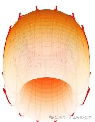
import numpy as np
import matplotlib.pyplot as plt
from mpl_toolkits.mplot3d import Axes3D  # Enable 3D support
from matplotlib import cm
# ==========================# 1. Initialize window# ==========================fig = plt.figure(figsize=(8, 7))
ax = fig.add_subplot(111, projection='3d')
ax.set_box_aspect((1, 1, 1))  # Equal proportions
ax.set_axis_off()             # Turn off axes
# Corresponding MATLAB: view(-30, 35)  ->  elev=35, azim=-30
ax.view_init(elev=35, azim=-30)
# ==========================# 2. Core Parameters# ==========================R = 4.0          # Major Radius
r_shell = 2.0    # Shell Radius
r_red = 1.95     # Red line radius
r_blue = 1.2     # Blue line radius (internal)
# ==========================# 3. Semi-transparent rainbow shell# ==========================num_pts = 120
theta, phi = np.meshgrid(    np.linspace(0, 2 * np.pi, num_pts),    np.linspace(0, 2 * np.pi, num_pts))
X = (R + r_shell * np.cos(phi)) * np.cos(theta)
Y = (R + r_shell * np.cos(phi)) * np.sin(theta)
Z = r_shell * np.sin(phi)
# Color mapping: Generate HSV rainbow based on phi
phase_shift = 3.5
C = np.mod(phi + phase_shift, 2 * np.pi)
C_norm = (C - C.min()) / (C.max() - C.min())  # Normalize to [0,1]
colors = cm.hsv(C_norm)
colors[..., 3] = 0.3  # alpha = 0.3, semi-transparent
surf = ax.plot_surface(    X, Y, Z,    facecolors=colors,    rstride=1, cstride=1,    linewidth=0,    antialiased=True,    shade=False  # We provided colors ourselves, no automatic shading)
# ==========================# 4. Red poloidal coils (E Field)# ==========================num_red_loops = 12
red_angles = np.linspace(0, 2 * np.pi, num_red_loops + 1)[:-1]
t = np.linspace(0, 2 * np.pi, 100)
for th in red_angles:    xr = (R + r_red * np.cos(t)) * np.cos(th)    yr = (R + r_red * np.cos(t)) * np.sin(th)    zr = r_red * np.sin(t)    ax.plot3D(xr, yr, zr, color=(0.8, 0, 0), linewidth=1.5)    # Add red arrows    arrow_indices = [20, 50, 80]    for idx in arrow_indices:        p = np.array([xr[idx], yr[idx], zr[idx]])        # Poloidal direction tangent vector (consistent with MATLAB formula, missing r is just a scalar, normalized is the same)
        vx = -np.sin(t[idx]) * np.cos(th)
        vy = -np.sin(t[idx]) * np.sin(th)
        vz =  np.cos(t[idx])
        vec = np.array([vx, vy, vz])
        vec = vec / np.linalg.norm(vec) * 0.6
        ax.quiver(            p[0], p[1], p[2],            vec[0], vec[1], vec[2],            length=1.0,            normalize=False,            color='r',            linewidth=2,            arrow_length_ratio=0.4  # Arrow head size        )
# ==========================# 5. Blue toroidal coils (H Field)# ==========================blue_phi_angles = [0, 0.5 * np.pi, np.pi, 1.5 * np.pi]
t_blue = np.linspace(0, 2 * np.pi, 200)
for phi_val in blue_phi_angles:    xb = (R + r_blue * np.cos(phi_val)) * np.cos(t_blue)    yb = (R + r_blue * np.cos(phi_val)) * np.sin(t_blue)    zb = r_blue * np.sin(phi_val) * np.ones_like(t_blue)    ax.plot3D(xb, yb, zb, 'c-', linewidth=2)    # Blue arrows    arrow_indices = range(15, 200, 30)    for idx in arrow_indices:        p = np.array([xb[idx], yb[idx], zb[idx]])        # Tangential vector along the large circle direction        vx = -np.sin(t_blue[idx])        vy =  np.cos(t_blue[idx])        vz = 0.0        vec = np.array([vx, vy, vz])        vec = vec / np.linalg.norm(vec) * 0.6        ax.quiver(            p[0], p[1], p[2],            vec[0], vec[1], vec[2],            length=1.0,            normalize=False,            color='c',            linewidth=2,            arrow_length_ratio=0.4        )
# ==========================# 6. Text Labels# ==========================ax.text(    R + r_shell + 0.5, 0, 1.5, 'E',    color='r', fontsize=24, fontweight='bold')
ax.text(    R + r_shell + 0.5, 0, -1.5, 'H',    color='c', fontsize=24, fontweight='bold')
ax.text(    0, -(R + r_shell), -3, 'F',    color='k', fontsize=20, fontweight='bold')
ax.set_title('Hybrid Toroidal Vortex', fontsize=18)
# ==========================# 7. View Range Adjustment# ==========================max_extent = R + r_shell + 1.0
ax.set_xlim(-max_extent, max_extent)
ax.set_ylim(-max_extent, max_extent)
ax.set_zlim(-max_extent, max_extent)
plt.tight_layout()
plt.show()
plt.savefig('/root/result.png')
print("Image saved to /root/result.png")