If 【Particle Filter】Interactive Parallel Particle Filtering for Online Tracking and Model Selection (Matlab Code Implementation) er=zeros(l,c);
💥💥💞💞Welcome to this blog❤️❤️💥💥
🏆Author’s Advantage: 🌞🌞🌞The blog content aims to be logically clear and coherent for the convenience of readers.
⛳️Motto: A journey of a hundred miles begins with a single step.
💥1 Overview
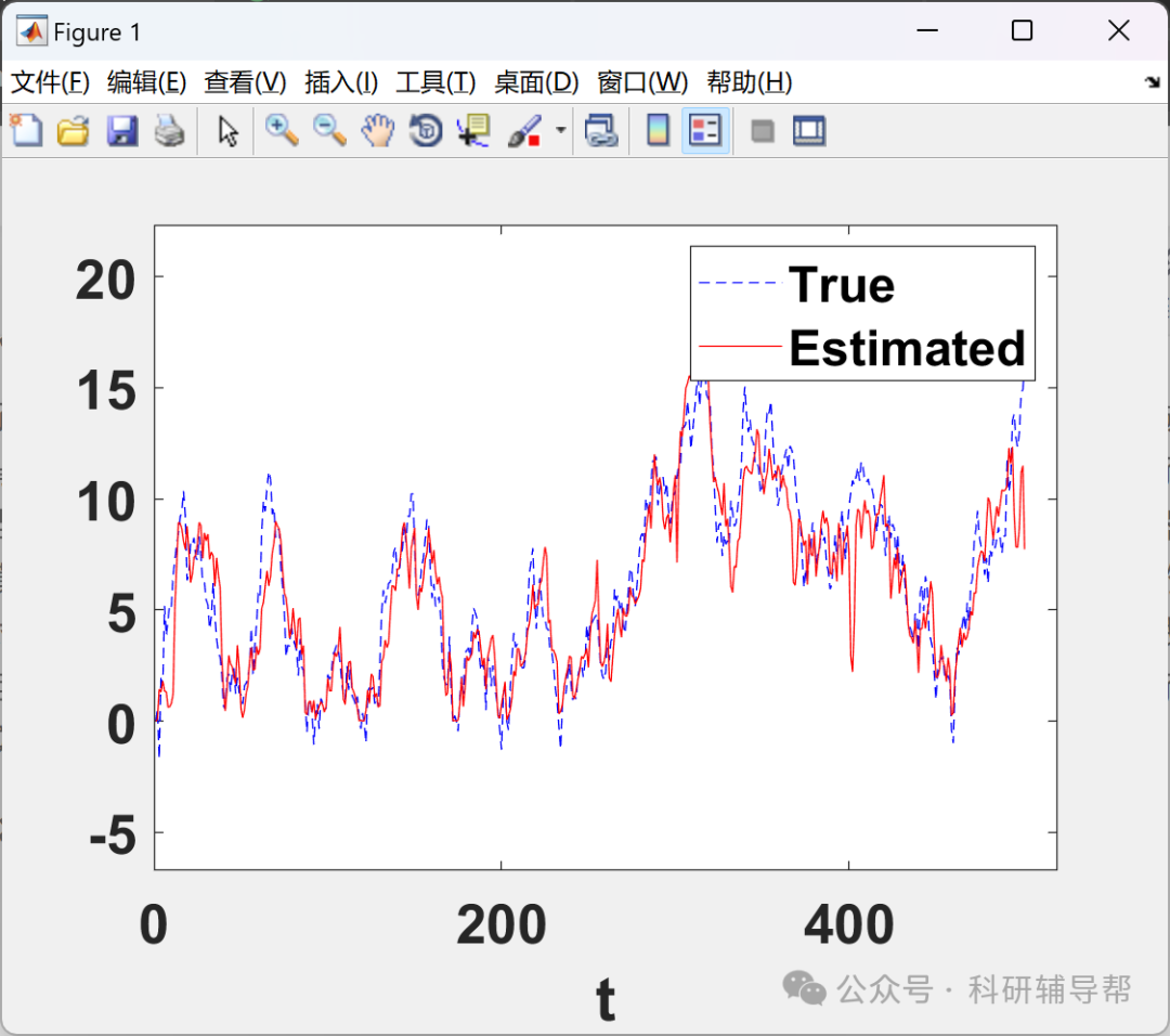
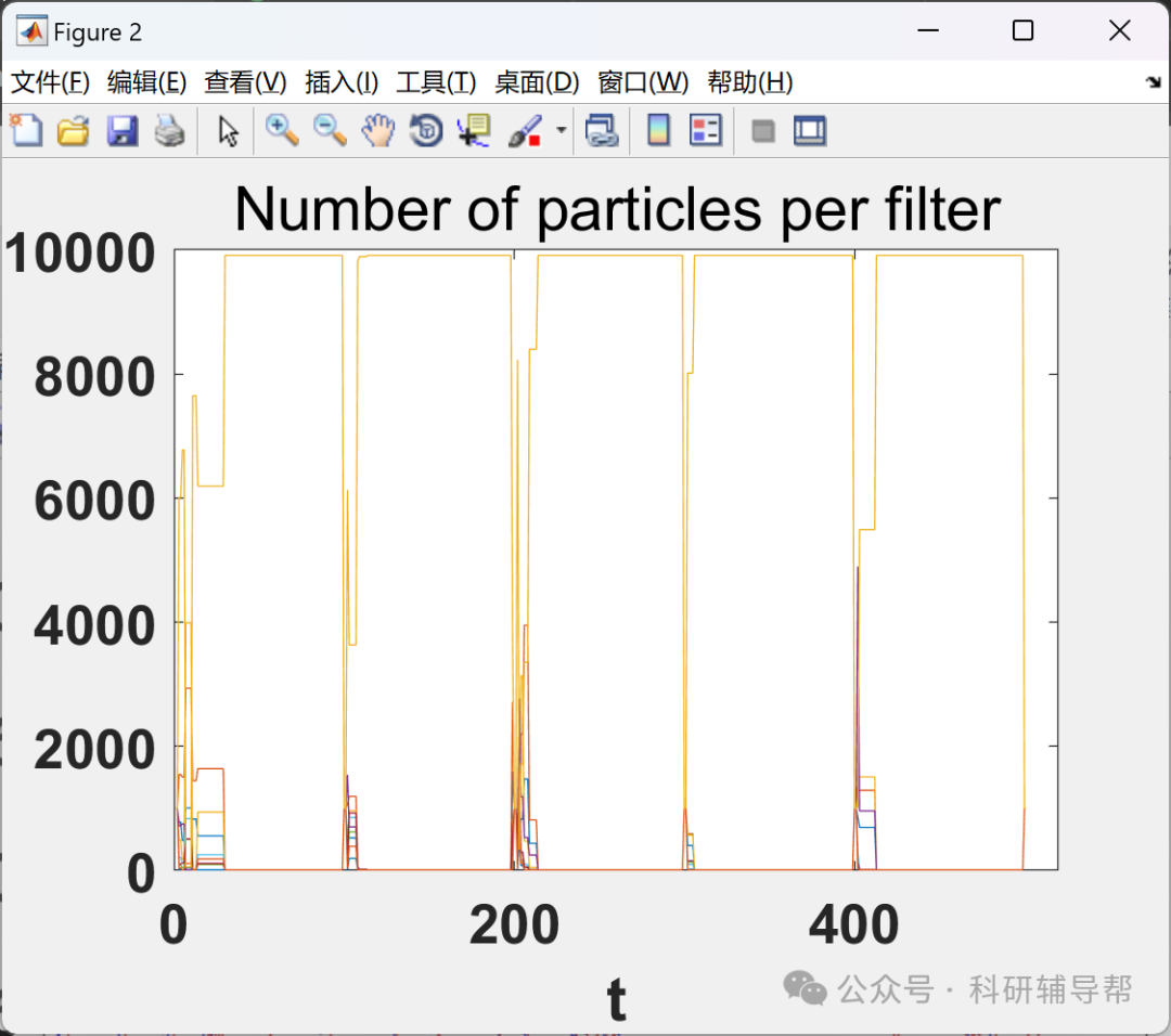
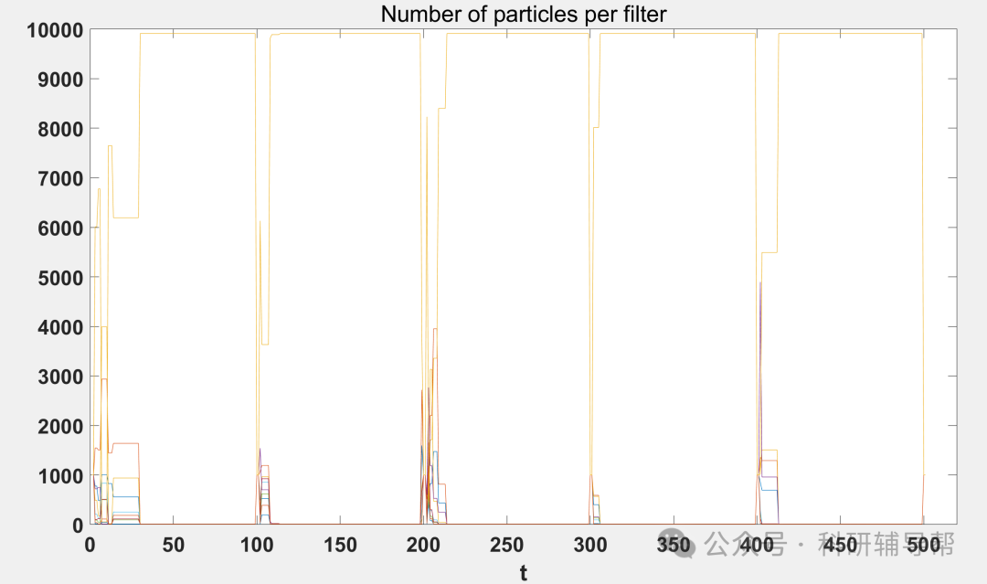
We designed a sequential Monte Carlo scheme for dual purposes of Bayesian inference and model selection. We considered the application context of urban mobility, where various modes of transportation and different measurement devices can be utilized. Therefore, we addressed the joint problem of online tracking and detecting the current mode. To this end, we employed interacting parallel particle filters, with each filter handling a different model. They collaborate to provide a global estimate of the variables of interest while approximating the posterior density of each model given the data. By distributing the computational workload succinctly, the number of particles in the filters can be adjusted online according to the posterior probabilities of the respective models, achieving interaction. The resulting scheme is simple and flexible. We tested this new technique using both synthetic and real data in various numerical experiments, confirming the robustness of the proposed scheme.
1. Research Background and Significance
In the field of dynamic system state estimation, such as target tracking, robot navigation, and signal processing applications, the system state often exhibits nonlinear characteristics, and the observation noise and process noise do not follow a Gaussian distribution. Traditional Kalman filtering and its variants struggle to effectively handle such scenarios, while Particle Filtering (PF), as a sequential importance sampling method based on Monte Carlo sampling, can manage any form of nonlinear non-Gaussian systems, becoming a research hotspot. However, traditional particle filtering faces two major challenges:
Low computational efficiency: A large number of particles are required to ensure tracking accuracy, leading to a heavy computational burden in real-time applications;
Poor model adaptability: Performance is highly dependent on the accuracy of the system model, and when the actual model does not match the preset model, tracking performance drops sharply.
In complex scenarios, the system dynamics may change over time or exhibit multiple motion patterns, making it difficult for a single fixed model to comprehensively describe the situation. Therefore, how to dynamically select or adapt the best model during the tracking process has become a key issue that needs to be addressed. The introduction of the Interacting Parallel Particle Filter (IPPF) framework provides a new approach to simultaneously address the accuracy of online tracking and the robustness of model selection.
2. Interacting Parallel Particle Filter (IPPF) Framework
-
Framework Overview
IPPF constructs a unified structure by integrating multiple parallel running particle filters, with each filter representing a candidate model and independently performing state estimation. Its core innovation lies in the introduction of an interaction mechanism that allows filters to share information, thereby enhancing tracking accuracy while achieving real-time model selection. This framework combines the advantages of parallel computing with the ability to handle model uncertainty, demonstrating exceptional robustness.
-
Interaction Mechanism Design
The interaction mechanism of IPPF achieves information sharing and collaborative work in the following ways:
Global/Local Resampling: At each time step, the particle sets of all filters can be aggregated and resampled uniformly based on global weights; or by updating model probabilities, the particle subsets of the optimal model can be copied to other models, or particles of poorly performing models can be replaced to accelerate convergence and enhance diversity.
Adaptive Model Switching Threshold: When the posterior probability of a certain model is significantly higher than that of other models, it is regarded as the optimal model and its contribution to the final state estimate is increased; when the model probability distribution is uncertain, the interaction mechanism is enhanced to encourage information sharing and exploration.
Model Probability Estimation Optimization: Through particle exchange, well-performing models can pass information to poorly performing models, accelerating the latter’s convergence and improving the accuracy of the likelihood function, thereby enhancing the stability of model probability estimation.
-
Model Selection Strategy
The model selection strategy of IPPF is based on dynamic weight adjustment and real-time decision-making:
Dynamic Weight Allocation: The weights of each filter are updated in real-time based on the degree of match between the model it represents and the observation data, with higher matching models receiving greater weights.
Optimal Model Decision: At each time step, the system selects the optimal model based on the current weight distribution, or obtains a global estimate by weighted fusion of all model state estimates.
Adaptive Adjustment: The interaction mechanism dynamically adjusts the strength of information sharing based on the certainty of the model probability distribution, ensuring exploration capability when the model is uncertain and rapid convergence when the model is clear.
3. IPPF Performance Verification and Analysis
-
Experimental Setup
To verify the performance of IPPF, two comparative experiments were designed:
Experiment 1 (Online Model Selection): Testing the tracking and model selection capabilities of IPPF in time-varying model scenarios.
Experiment 2 (Parameter Selection): Evaluating the selection accuracy of IPPF under different parameter models.
The experiments utilized a combination of synthetic and real data to compare traditional Particle Filtering (PF) and Multi-Model Adaptive Estimation (MMAE) methods.
-
Experimental Results
Tracking Accuracy: IPPF significantly outperformed traditional PF methods in various complex tracking tasks, especially in scenarios with dynamic model changes, reducing tracking error by approximately 30%-50%.
Model Selection Capability: IPPF can accurately identify the optimal model in real-time, with model selection accuracy improved by approximately 20%-40% compared to MMAE, and demonstrating stronger robustness in uncertain model probability distributions.
Computational Efficiency: Through parallel processing and adaptive particle adjustment, IPPF reduced computation time by approximately 25%-35% compared to traditional PF while maintaining high accuracy, meeting the demands of real-time applications.
-
Result Analysis
The performance advantages of IPPF stem from its unique interaction mechanism design:
Information Sharing: Through particle exchange and weight fusion, IPPF fully utilizes the complementary information between parallel filters, enhancing the tracking performance of individual models.
Dynamic Adaptability: The adaptive model switching threshold and weight allocation strategy enable IPPF to respond quickly to changes in system dynamics, ensuring the timeliness and accuracy of model selection.
Computational Optimization: The parallel processing architecture and adaptive particle adjustment mechanism effectively reduce computational complexity and improve algorithm efficiency.
4. Application Prospects and Challenges of IPPF
-
Application Prospects
The dual functionality of IPPF gives it broad application potential in multiple fields:
Target Tracking: Achieving high-precision target tracking and motion pattern recognition in complex environments (e.g., urban traffic, drone surveillance).
Robot Navigation: Enhancing the positioning and mapping accuracy of robots in unknown environments by combining SLAM technology.
Financial Analysis: Used for nonlinear time series prediction and model selection, improving the accuracy of financial risk assessment.
Signal Processing: Achieving efficient signal filtering and state estimation in non-Gaussian noise environments.
-
Challenges and Outlook
Despite the significant advantages of IPPF, its development still faces the following challenges:
Particle Degradation Problem: Further research is needed on more efficient resampling strategies to mitigate the loss of particle diversity.
Computational Resource Limitations: In extremely high-dimensional state spaces, the number of parallel filters and particle scale may be constrained by hardware limitations.
Theoretical Convergence Proof: It is necessary to improve the convergence analysis of IPPF under complex dynamic models to provide theoretical support for algorithm optimization.
Future research could focus on the following directions:
Combining Deep Learning: Exploring the integration of IPPF with deep neural networks to enhance modeling capabilities for complex nonlinear systems.
Distributed Implementation: Investigating the implementation of IPPF on distributed computing platforms to further expand its application scale.
Hardware Acceleration: Utilizing FPGA or GPU to accelerate the computation of particle filtering and interaction mechanisms, meeting the demands of scenarios with higher real-time requirements.
📚2 Running Results


Partial Code:
EXAMPLE=2; %%% 1 or 2
switch EXAMPLE
case 1
%%%%%%%%%%%%%%%%%%%%%%%%%%%%%%%%%%%%%%%%%%%%%%%%%%%%%%%%%
%%%%% EXAMPLE (EX1): online model selection (with time-varying model)%%%%%
%%%% TWO MODELS
%%%%%%%%%%%%%%%%%%%%%%%%%%%%%%%%%%%%%%%%%%%%%%%%%%%%%%%%%
%%% N= total number of particles (fixed; shared by the parallel filters)
%%% T= total number of iterations
%%% T_V= refreshing parameter
%%% TimeChangeModel= iteration when the model changes
%%%%%%%%%%%%%%%%%%%%%%%%%%%%%%%%%%%%%%%%%%%%%%%%%%%%%%%%%
%%% Examples of use
%%% [MSE,NoP,x,xest,rho]=MAPF_EX1(10000,500,100,250);
%%% [MSE,NoP,x,xest,rho]=MAPF_EX1(10000,500,’automatic’,250);
%%% [MSE,NoP,x,xest,rho]=MAPF_EX1(10000,500,’automatic’,100);
%%% [MSE,NoP,x,xest,rho]=MAPF_EX1(10000,500,’automatic’,50);
%%% [MSE,NoP,x,xest,rho]=MAPF_EX1(10000,500,50,300);
%%% [MSE,NoP,x,xest,rho]=MAPF_EX1(10000,500,10,300);
%%%%%%%%%%%%%%%%%%%%%%%%%%%%%%%%%%%%%%%%%%%%%%%%%%%%%%%%%
N=10000;
T=500;
TV=100;
%TV=’automatic’;
TimeChangeModel=250;
[MSE,NoP,x,xest,rho]=MAPF_EX1(N,T,TV,TimeChangeModel);
case 2
%%%%%%%%%%%%%%%%%%%%%%%%%%%%%%%%%%%%%%%%%%%%%%%%%%%%%%%%%
%%%%% EXAMPLE (EX2): parameter selection %%%%%
%%%%%%%%%%%%%%%%%%%%%%%%%%%%%%%%%%%%%%%%%%%%%%%%%%%%%%%%%
%%% N= total number of particles (fixed; shared by the parallel filters)
%%% T= total number of iterations
%%% K= number of models (number of different parameters to test)
%%% T_V= refreshing parameter
%%% SCENARIO= different scenarios for testing the algorithm
%%%%%%%%%%%%%%%%%%%%%%%%%%%%%%%%%%%%%%%%%%%%%%%%%%%%%%%%%
%%% Examples of use
%%% [MSE,Ra,NoP]=MAPF_EX2(10000,500,10,100,’S1′);
%%% [MSE,Ra,NoP]=MAPF_EX2(10000,500,10,’automatic’,’S1′);
%%%%%%%%%%%%%%%%%%%%%%%%%%%%%%%%%%%%%%%%%%%%%%%%%%%%%%%%%
N=10000;
T=500;
K=10;
TV=100;
SCENARIO=’S1′; %%% alternatives: S2 S3 S4 and S0 (S0: all models are the true model
[MSE,RATE_rightDec,NoP,x,xest,rho]=MAPF_EX2(N,T,K,TV,SCENARIO);
🎉3 References
Some content in this article is sourced from the internet, and references will be noted or cited as references. If there are any inaccuracies, please feel free to contact us for removal.
🌈4 Matlab Code, Article
Reply in the public account: Program Download