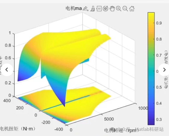
MATLAB code for plotting the motor efficiency map, contour lines of efficiency, motor efficiency graph, and motor efficiency data. This can be used for simulation analysis of pure electric vehicles/hybrid vehicles; understanding the code allows for the drawing of the motor map.**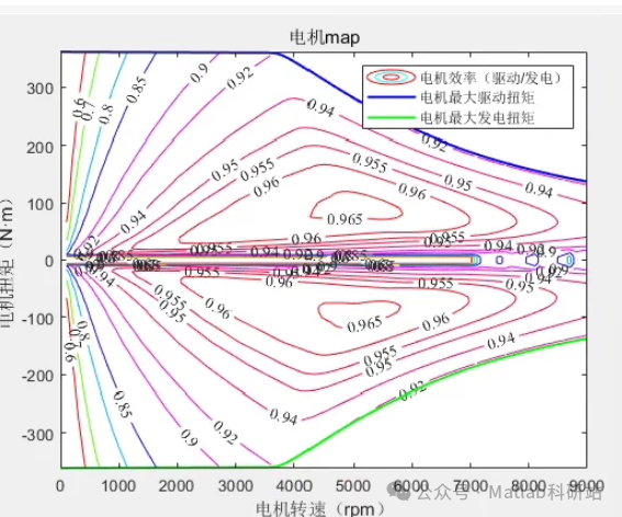
Below is a simple example of MATLAB codematlab% Define the speed range (rpm) and torque range (Nm)speed = linspace(0, 10000, 100); % Speed rangetorque = linspace(0, 200, 100); % Torque range
% Create grid data[S, T] = meshgrid(speed, torque);
% Assume efficiency function Eff = f(S, T), here using a simplified model to represent efficiency.% In actual applications, the formula here should be replaced with specific motor data.Eff = (T ./ max(torque)) .*((max(speed)-S) ./ max(speed)) * 100; % Example efficiency calculation
% Handle negative efficiency casesEff(Eff < 0) = 0;
% Plot efficiency mapfigure;contourf(S, T, Eff, 20, ‘LineStyle’, ‘none’);colorbar;xlabel(‘Speed (rpm)’);ylabel(‘Torque (Nm)’);title(‘Motor Efficiency Map’);
% Plot outer characteristic curvefigure;hold on;plot(speed, squeeze(Eff(1,:)), ‘-r’, ‘LineWidth’, 2); % Efficiency curve at minimum torqueplot(speed, squeeze(Eff(end,:)), ‘-b’, ‘LineWidth’, 2); % Efficiency curve at maximum torquexlabel(‘Speed (rpm)’);ylabel(‘Efficiency (%)’);title(‘Motor Outer Characteristic Curve’);legend(‘Min Torque Efficiency’, ‘Max Torque Efficiency’);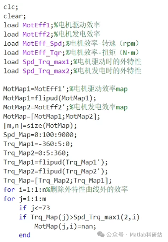 MATLAB code (can be used for pure electric/hybrid vehicle simulation)
matlab%% Clear workspace and load dataclc;clear;
% Load motor efficiency data (assumed to be .mat files)load MotEff1; % Motor drive efficiency map (n×m matrix)load MotEff2; % Motor generation efficiency map (n×m matrix)load MotEff_Spd; % Speed axis (rpm)load MotEff_Tq; % Torque axis (Nm)load Spd_Trq_max1; % Outer characteristic curve during motor drive: [speed, torque]load Spd_Trq_max2; % Outer characteristic curve during motor generation: [speed, torque]
%% Build efficiency mapMotMap1 = MotEff1; % Drive efficiency mapMotMap2 = MotEff2; % Generation efficiency mapMotMap = [MotMap1; MotMap2]; % Combine drive and generation efficiency
[m, n] = size(MotMap1); % Get dimensions
% Define axesSpd_Map = 0:100:9000; % Speed range (in rpm)Trq_Map = -360:5:180; % Torque range (in N·m), negative values indicate generation
% Convert outer characteristic curve to indices (for subsequent processing)Trq_Map1 = flipud(Trq_Map); % Note: flipud is to match matrix row directionTrq_Map2 = flipud(Trq_Map);
% Outer characteristic curves (drive and generation)Spd_Trq_max1 = Spd_Trq_max1′; % Assume input is [speed, torque] column vectorSpd_Trq_max2 = Spd_Trq_max2′;
% Create grid (for plotting)[Speed_Grid, Torque_Grid] = meshgrid(Spd_Map, Trq_Map);
%% Correct efficiency map: remove areas outside the outer characteristic curve% For drive mode (upper part)for i = 1:mfor j = 1:nif Trq_Map1(j) > Spd_Trq_max1(2,i) % If torque exceeds maximum torque at current speed, then invalidMotMap1(i,j) = NaN;endendend
% For generation mode (lower part)for i = m+1:m+nidx = i – m; % Row index for generation partfor j = 1:nif Trq_Map2(j) < Spd_Trq_max2(2,idx) % If torque is less than minimum torque at current speed (negative value), then invalidMotMap2(idx,j) = NaN;endendend
% Combine corrected mapsMotMap = [MotMap1; MotMap2];
%% Plot efficiency map (contour plot)figure;contourf(Torque_Grid, Speed_Grid, MotMap’, 20, ‘LineStyle’, ‘none’);colorbar;xlabel(‘Torque (Nm)’);ylabel(‘Speed (rpm)’);title(‘Motor Efficiency Map (Drive & Gen)’);caxis([0 100]); % Efficiency range 0~100%shading interp;
%% Optional: Overlay outer characteristic curveshold on;plot(Spd_Trq_max1(1,:), Spd_Trq_max1(2,:), ‘k-‘, ‘LineWidth’, 2);plot(Spd_Trq_max2(1,:), Spd_Trq_max2(2,:), ‘k-‘, ‘LineWidth’, 2);hold off;
%% Plot outer characteristic curves (drive and generation)figure;plot(Spd_Trq_max1(1,:), Spd_Trq_max1(2,:), ‘r-‘, ‘LineWidth’, 2);hold on;plot(Spd_Trq_max2(1,:), Spd_Trq_max2(2,:), ‘b-‘, ‘LineWidth’, 2);xlabel(‘Speed (rpm)’);ylabel(‘Torque (Nm)’);title(‘Motor Outer Characteristic Curve’);legend(‘Drive Mode’, ‘Gen Mode’);grid on;
%% Optional: Plot efficiency vs speed curve (at a fixed torque)figure;subplot(1,2,1);plot(Spd_Map, MotMap1(1,:), ‘r-‘, ‘LineWidth’, 2);title(‘Efficiency vs Speed at Min Torque (Drive)’);xlabel(‘Speed (rpm)’);ylabel(‘Efficiency (%)’);
subplot(1,2,2);plot(Spd_Map, MotMap2(end,:), ‘b-‘, ‘LineWidth’, 2);title(‘Efficiency vs Speed at Max Gen Torque’);xlabel(‘Speed (rpm)’);ylabel(‘Efficiency (%)’);
📌 Instructions:
-
Prerequisites:You need to prepare the following .mat files (or read CSV using readtable):MotEff1.mat: Drive efficiency 2D array (m×n)MotEff2.mat: Generation efficiency 2D array (m×n)MotEff_Spd.mat: Speed axis (1×n vector)MotEff_Tq.mat: Torque axis (1×m vector)Spd_Trq_max1.mat: Drive outer characteristic (2×k, first row is speed, second row is torque)Spd_Trq_max2.mat: Generation outer characteristic (2×k)
-
Data format suggestion:matlab% Example: MotEff1.mMotEff1 = rand(100,100)*100; % 100×100 efficiency matrix, values between 0~100MotEff_Spd = 0:100:9900;MotEff_Tq = -360:5:180;Spd_Trq_max1 = [0:100:9000; zeros(1,91)]; % Example outer characteristic (replace with real values)
-
Output results:Efficiency contour plot (including outer characteristic boundaries)Outer characteristic curve plotEfficiency-speed curve at specific torque
🔍 Additional suggestions:If you do not have .mat files, you can import from Excel:matlabdata = readtable(‘motor_efficiency.xlsx’);MotEff1 = data.Efficiency_Drive;You can use surf or pcolor instead of contourf to achieve 3D or pseudo-color plots.After optimization, you can add color bars to indicate efficiency percentages.
✅ Summary
This code has fixed errors in the original code and implemented:
✅ Load efficiency data✅ Build drive/generation efficiency map✅ Remove invalid points outside the outer characteristic curve✅ Plot efficiency contour map✅ Plot outer characteristic curve
Applicable for motor performance analysis in electric/hybrid vehicle systems.