
Long time no see, friends. In the last issue, we shared various statistical measures in MATLAB. In this issue, we will share how to call functions for seven common distributions in MATLAB.
In probability statistics, there are seven commonly used distribution functions: Binomial distribution, Poisson distribution, Normal distribution, Uniform distribution, Chi-square distribution, t-distribution, and F-distribution.
Part.01
Binomial Distribution
The Binomial Distribution is a common discrete probability distribution in statistics. If an event is subjected to n independent trials (Bernoulli trials), and the probability of event A occurring in each trial is p, then the probability of event X=k, which means “event A occurs exactly k times in n trials,” is given by:
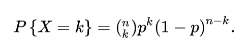
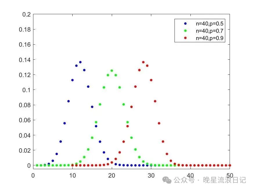
If the random variable X follows a Binomial distribution with parameters n and p, we denote it as X ~ B(n, p). The expectation (mean) of the Binomial distribution is E(X)=np, and the variance is D(X)=np(1-p). The graph of the Binomial distribution is approximately as follows:
In MATLAB, you can use the function binopdf(x,n,p) to represent the probability density function of the Binomial distribution, which directly generates the probability at the corresponding point. In the function, x represents the point of interest, n represents the total number of Bernoulli trials, and p represents the probability of each Bernoulli trial:
clc
clear
close all

data1=binopdf(5,10,0.5)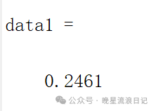
If the first parameter is a vector, the generated probabilities will also be a vector:
clc
clear
close all

data2=binopdf(1:40,40,0.3);
plot(1:40,data2,'o','MarkerSize',3.5,'MarkerFaceColor','blue','MarkerEdgeColor','blue')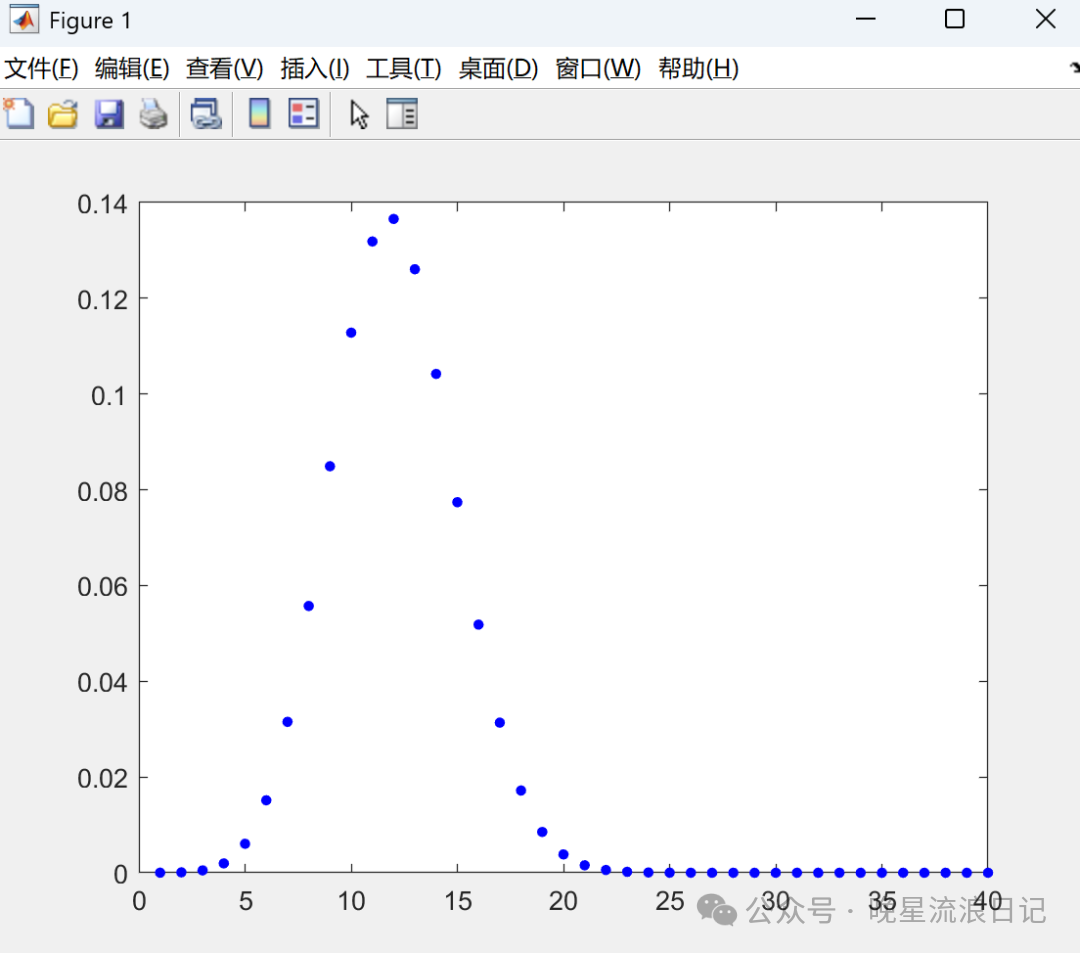
The above calculates the probability of a specific point. If you want to calculate the probability over a range, for example, the probability of success being less than 5 times in 10 Bernoulli trials, you can use the cumulative distribution function binocdf(x,n,p) to solve it, where n and p are the same as before, and x represents the range of counts less than x:
clc
clear
close all

data3=binocdf(5,10,0.5)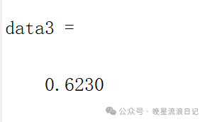
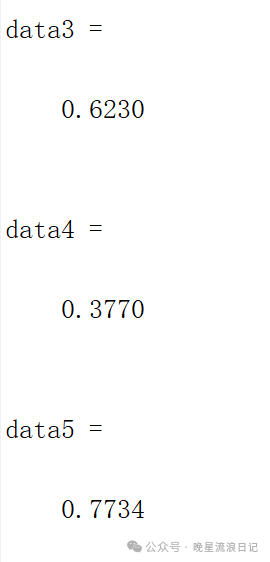
If you want to calculate the greater part, just use 1-; if you want to calculate a specific range, you need to use two binocdf() functions together:
clc
clear
close all

data3=binocdf(5,10,0.5)

data4=1-binocdf(5,10,0.5)

data5=binocdf(7,10,0.5)-binocdf(3,10,0.5)
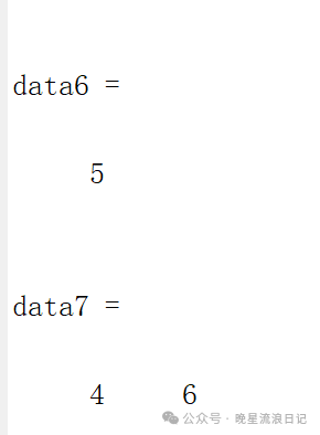
If we know the probability and want to find the corresponding count, we usually use the inverse cumulative distribution function. In MATLAB, the inverse cumulative distribution function for the Binomial distribution is binoinv(y,n,p), where n and p are the same as before, and y represents the probability sought.
clc
clear
close all

data6=binoinv(0.5,10,0.5)
data7=binoinv([0.3,0.7],10,0.5)
For the above examples, in reality, the values must be greater than 0, and the probabilities must be between 0 and 1 to have practical significance. However, MATLAB calculates these data using numerical methods, so even if there is no practical significance, MATLAB will still provide a corresponding value or use NAN to indicate that the result does not exist, and will not directly report an error. Therefore, when using these functions, it is important to pay special attention to whether the input data is correct.
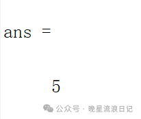
Finally, if you want to generate random numbers that follow a Binomial distribution in MATLAB, you can use binornd(n,p,a,b), where a and b indicate that the generated random numbers form a matrix with a rows and b columns. Note that the generated random numbers represent the number of repetitions of the Bernoulli trials, and when the quantity is sufficiently large, the numbers appearing near the mean will be significantly higher than those in other positions:
clc
clear
close all

data8=binornd(10,0.5,1,100);
mode(data8)
This concludes the applications of the Binomial distribution in MATLAB. The usage of other probability density functions in MATLAB is similar, and I will not elaborate further, just provide a brief introduction.
Part.02
Poisson Distribution
The Poisson distribution is an important discrete distribution. The Poisson distribution can be seen as the limit of the Binomial distribution. If the number of trials n in the Binomial distribution is large, the probability p is small, and the product λ=np is moderate, then the probability of the occurrence of an event can be approximated by the Poisson distribution.
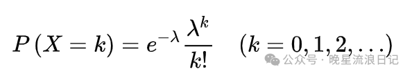
If the random variable X follows a Poisson distribution with parameter λ, where λ > 0, it is denoted as X~π(λ) or X~Poisson(λ). In the Poisson distribution, λ is the only parameter, which is both the mathematical expectation and the variance. Its probability density function is:
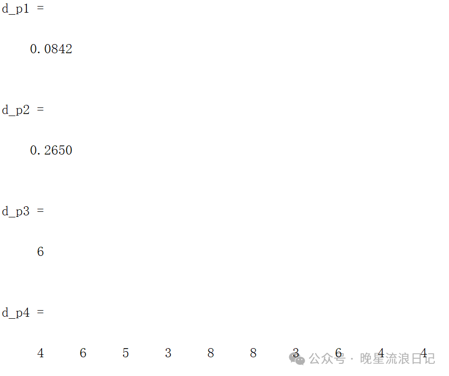
In MATLAB, you can use the following functions to solve for the required values: poisspdf() for the probability density function, poisscdf() for the cumulative distribution function, poissinv() for the inverse cumulative distribution function, and poissrnd() for the random number generator:
clc
clear
close all

% poisson
d_p1=poisspdf(2,5)
d_p2=poisscdf(3,5)
d_p3=poissinv(0.75,5)
d_p4=poissrnd(5,1,10)
Part.03
Normal Distribution
The Normal distribution, also known as the Gaussian distribution, is a continuous distribution that can be seen as the continuous form of the Binomial distribution. Mathematically, it is denoted as X~N(μ,σ²), where μ is the mathematical expectation (mean) of the Normal distribution, and σ² is the variance of the Normal distribution. The Normal distribution with μ = 0 and σ = 1 is called the standard normal distribution, and its probability density function is:

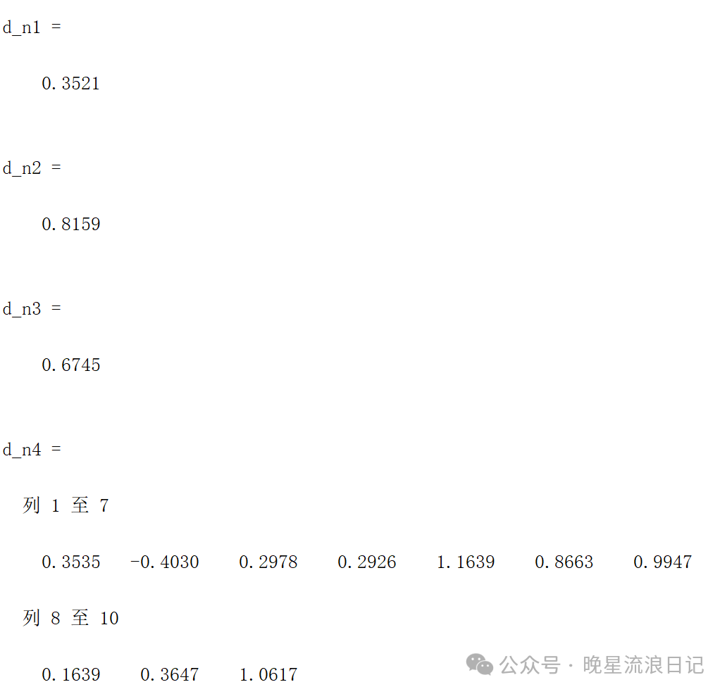
In MATLAB, you can use the following functions to solve for the required values: normpdf() for the probability density function, normcdf() for the cumulative distribution function, norminv() for the inverse cumulative distribution function, and normrnd() for the random number generator:
clc
clear
close all

% normal
d_n1=normpdf(0.5,0,1)
d_n2=normcdf(0.9,0,1)
d_n3=norminv(0.75,0,1)
d_n4=normrnd(0,1,1,10)
Part.04
Uniform Distribution
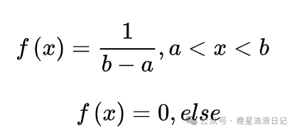
The Uniform distribution is a continuous probability distribution defined over the interval [a, b], where the probability of any point is the same, and the boundary values do not affect the integral result. Mathematically, it is denoted as U(a,b), with the expected value being (a+b)/2 and the variance being (b−a)²/12. Its probability density function is:
In MATLAB, you can use the following functions to solve for the required values: unifpdf() for the probability density function, unifcdf() for the cumulative distribution function, unifinv() for the inverse cumulative distribution function, and unifrnd() for the random number generator:
clc
clear
close all
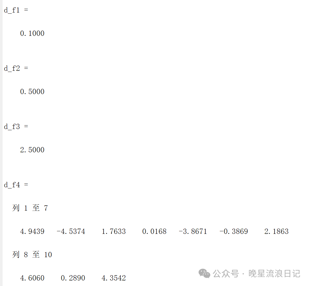
% uniform
d_f1=unifpdf(3,-5,5)
d_f2=unifcdf(0,-5,5)
d_f3=unifinv(0.75,-5,5)
d_f4=unifrnd(-5,5,1,10)
Part.05
Three Major Sampling Distributions
The three major sampling distributions are the Chi-square distribution, t-distribution, and F-distribution.
The Chi-square distribution (chi-square distribution) states that if n independent random variables ξ₁, ξ₂, …, ξn follow a standard normal distribution, then the sum of the squares of these n standard normal random variables forms a new random variable, and its distribution is called the Chi-square distribution, denoted as X~c²(n).
If the random variable X follows a standard normal distribution, and Y follows a Chi-square distribution with n degrees of freedom, then Z=X/(Y/n)^(1/2) follows a t-distribution, denoted as Z~t(n).
If the random variable X₁ follows a Chi-square distribution with n degrees of freedom, and X₂ follows a Chi-square distribution with m degrees of freedom, then Y=(X₁/n)/(X₂/m) follows an F-distribution, denoted as Y~F(n,m).
In MATLAB, you can use the following functions to solve for the required values. For the Chi-square distribution: chi2pdf() for the probability density function, chi2cdf() for the cumulative distribution function, chi2inv() for the inverse cumulative distribution function, and chi2rnd() for the random number generator. For the t-distribution: tpdf() for the probability density function, tcdf() for the cumulative distribution function, tinv() for the inverse cumulative distribution function, and trnd() for the random number generator. For the F-distribution: fpdf() for the probability density function, fcdf() for the cumulative distribution function, finv() for the inverse cumulative distribution function, and frnd() for the random number generator:
clc
clear
close all
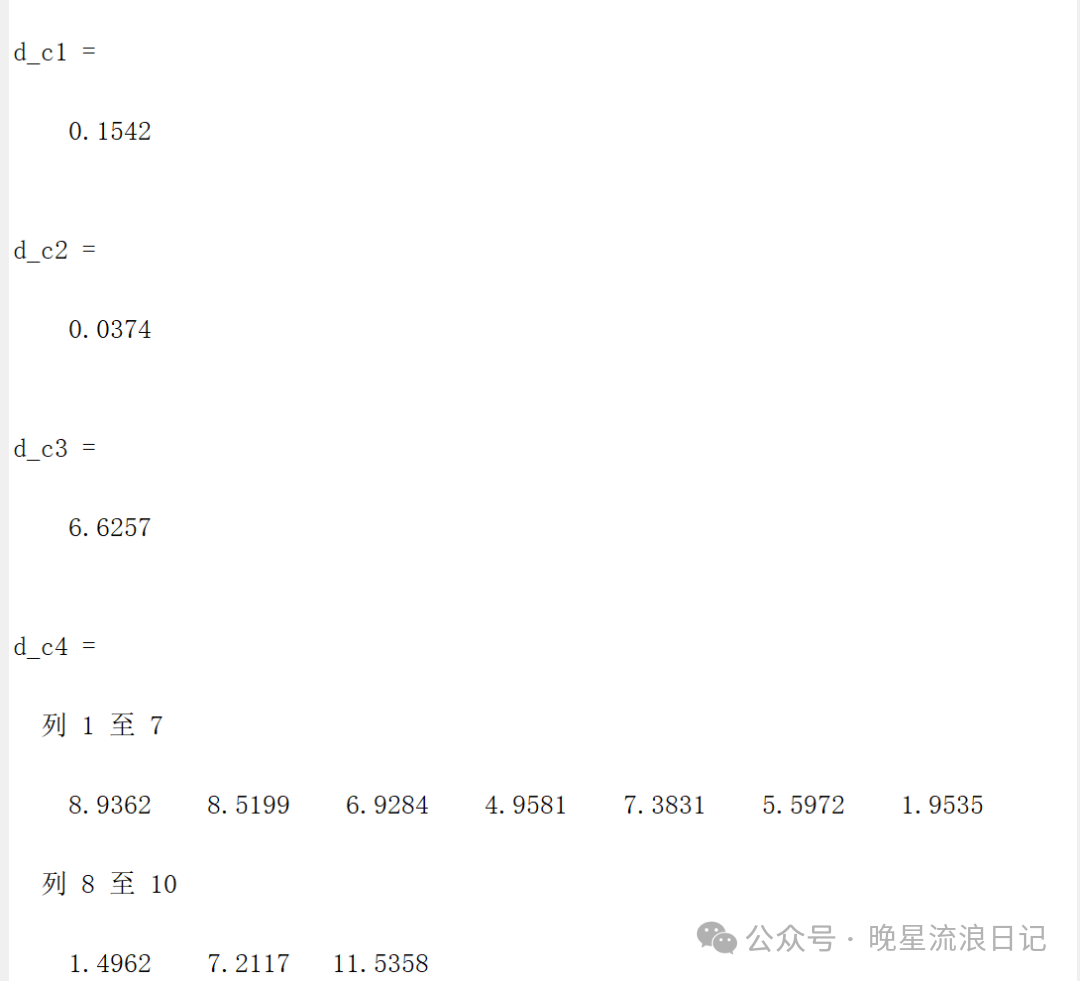
% Chi-square distribution
d_c1=chi2pdf(3,5)
d_c2=chi2cdf(1,5)
d_c3=chi2inv(0.75,5)
d_c4=chi2rnd(5,1,10)
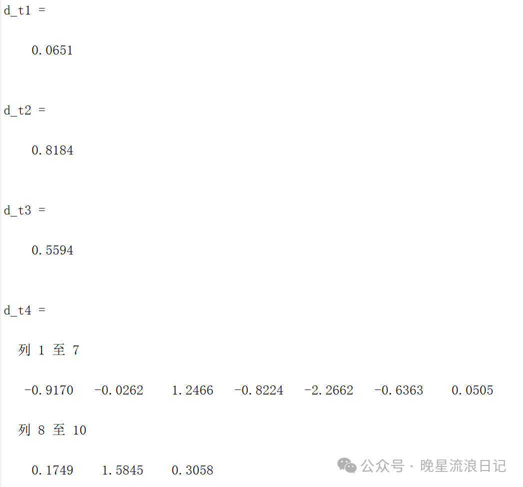
% t-distribution
d_t1=tpdf(2,5)
d_t2=tcdf(1,5)
d_t3=tinv(0.7,5)
d_t4=trnd(5,1,10)
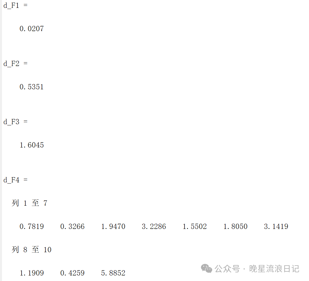
% F-distribution
d_F1=fpdf(5,3,5)
d_F2=fcdf(1,3,5)
d_F3=finv(0.7,3,5)
d_F4=frnd(3,5,1,10)
In fact, from here on, the usage is very similar to the initial Binomial distribution; you just need to input the quantity to be solved, then input the corresponding distribution parameters, and even the corresponding functions only need to modify the prefix, while the suffix remains the same.
Today’s sharing ends here. In the next issue, we will share the third part of statistical analysis—parameter estimation and hypothesis testing. See you next time.

END
Click below
Follow us