In seismic signal processing, spectrum analysis is one of the commonly used signal analysis techniques. As a drawing technique tutorial, this article provides a visual display of seismic data, single-trace recorded waveforms, and their spectrum.
In fact, seismic waveform displays are usually drawn by filling the area of a half-polar closed curve, which can be achieved using the <span>fill</span> function in MATLAB. The spectrum analysis curve can assist in shadow filling to enhance the visual effect.
1. Drawing Example
Given seismic data with a sampling rate of 2ms and a duration of 500ms, totaling 301 traces, we will plot a 2-D pseudo-color seismic profile, single-trace seismic record, and spectrum graph.
The implementation code is as follows:
%=========================================================================
% DEMO: Seismic signal analysis
%
% Parameter description:
%    nsamps: sample numbers
%    ntrace: trace numbers
%    dt:     sampling time
%    fs:     sampling frequency
%    nfft:   FFT points
%    df:     frequency space
%    Author: Peng Zhenming
%    School of Information and Communication Engineering,
%    University of Electronic Science and Technology of China
%    http://idiplab.uestc.cn/
%    Date: 2015.12.26,
%
% Revised: 2025.08.27
%=========================================================================
clc, clear, close all;
%=========================================================================
dt = 2.0;      % Sampling time: Millisecond

%=========================================================================
% Read the seismic data from text file
y = importdata('seismic_nsamp251_tr301_2ms.txt');
%==========================================================================

[nsamps, ntrace] = size(y);
y = y/max(y(:));
imagesc(imadjust(y));      % imagesc(y(1:nsamps,1:ntrace));
colormap(diyCM(18,256))  % diyCM Colors
% colormap(jet);

colorbar

t = dt*(0:nsamps-1);       % Millisecond

tick = floor(linspace(0, nsamps-1, 6)); % Number of marked points
yticks(tick);                         % Number of marked points
yticklabels(string(dt*tick));         % Label text

% Figure size and position
set(gcf, 'Unit', 'Centimeters', 'Position', [12, 8, 24, 12])
set(gcf, 'Color', 'White');             %  White Background

xlabel('Trace no'); ylabel('Time/ms');
set(gca, 'XAxisLocation', 'top');       % x-axis ticks on top
xlim([0 max(ntrace)]), ylim([0 max(nsamps)])
%==========================================================================

traceid = 1;             % Select trace number
% traceid = round(traceid);
traceid(traceid < 1)      =  1;
traceid(traceid > ntrace) =  ntrace;

s = y(:, traceid);        % Get a seismic trace
s1 = s; s1(s1 <= 0) = 0;  % Remain positive
s2 = s; s2(s2 > 0) = 0;  % Remain negative

figure,
set(gcf, 'Unit', 'Centimeters', 'Position', [20, 8, 4, 12])

area(t, s1, 'FaceColor', 'b', 'EdgeColor', 'b', 'FaceAlpha', 0.6); hold on
% area(t, s2, 'FaceColor', 'b', 'EdgeColor', 'k', 'FaceAlpha', 0.6);
% plot(t, s2, 'k', 'LineWidth', 1.2);
plot(t, s, 'b')

% seisViewer(s, 0.1, 'k', 'k')

set(gca, 'ydir', 'reverse')
xlabel('Time/ms');
ylabel('Trace no');
% set(gca, 'XAxisLocation', 'top');                  % x-axis ticks on top
set(gca, 'YAxisLocation', 'right', 'YTickLabel', '');  % y-axis ticks on right
grid on
view(-90, -90)

%==========================================================================
nfft = nsamps;                 % FFT using data points
fs = 1/dt;
df = 1000*fs/(nfft-1);         % Frequency spacing/Precision
f = df*(0:(nfft-1)/2);         % Physical frequency/Unilateral spectrum
%==========================================================================

Fs = fft(s, nfft);
amp = abs(Fs(1:floor(nfft/2)+1))/max(abs(Fs(:)));  % Normalization

figure,
% Figure size and position
set(gcf, 'Unit', 'Centimeters', 'Position', [24, 8, 24, 12])
set(gcf, 'Color', 'White');    %  White Background

% Set parameters
color = [0, 0.4470, 0.7410]; % [0.85, 0.33, 0.10]
alpha = 0.65;
lineWidth  = 0.80;

patchshade(f, amp, color, alpha, lineWidth);  % Patches for the shaded region
% area(f, amp, 'FaceColor', 'g'), hold on
% plot(f, amp', 'LineWidth', 1.2);

xlabel('Frequency/Hz'); ylabel('Amplitude(Normalized)');
xlim([0 max(f)]);
grid on

% Figure decoration
defaultAxes
2. Shadow Filling
The following code provides a curve plotting function for gradient shadow filling, <span>patchshade</span>, and other calling functions can be downloaded from the attachment.
function patchshade(x, y, color_value, alpha_value, line_width)
%-----------------------------------------------------------
% Create patches for the shaded region
narginchk(0, 5)
% ----------------
ax = gca;

if nargin < 2
    error('Please input the x and y vectors!');
end

if nargin < 3 || isempty(color_value)
    color_value = ax.ColorOrder(ax.ColorOrderIndex, :);  % Default color
end

if nargin < 4 || isempty(alpha_value)
    alpha_value = 0.15;                                 % Default alpha
end

if nargin < 5 || isempty(alpha_value)
    line_width = 2.0;                                   % Default Width
end

y_min = min(y);
y_max = max(y);
V_alpha = alpha_value * ((y - y_min) / y_max);
F = [1 2 3 4];

hold on
for k = 1:numel(x)-1
    V = [ x(k) y_min; x(k) y(k); x(k+1) y(k+1); x(k+1) y_min ];
    A = [0, V_alpha(k), V_alpha(k+1), 0]';
    patch('Faces', F, 'Vertices', V, 'FaceColor', color_value,
        'EdgeColor', 'none',
        'FaceVertexAlphaData', A, 'FaceAlpha', 'interp',
        'AlphaDataMapping', 'none');
end

hold on
plot(x, y, 'LineWidth', line_width, 'Color', color_value);
end
The above is a general drawing function for shadow-filled curves, which can be directly called for other purposes of curve display.
Loading seismic (text format) data, the program runs with the following results.
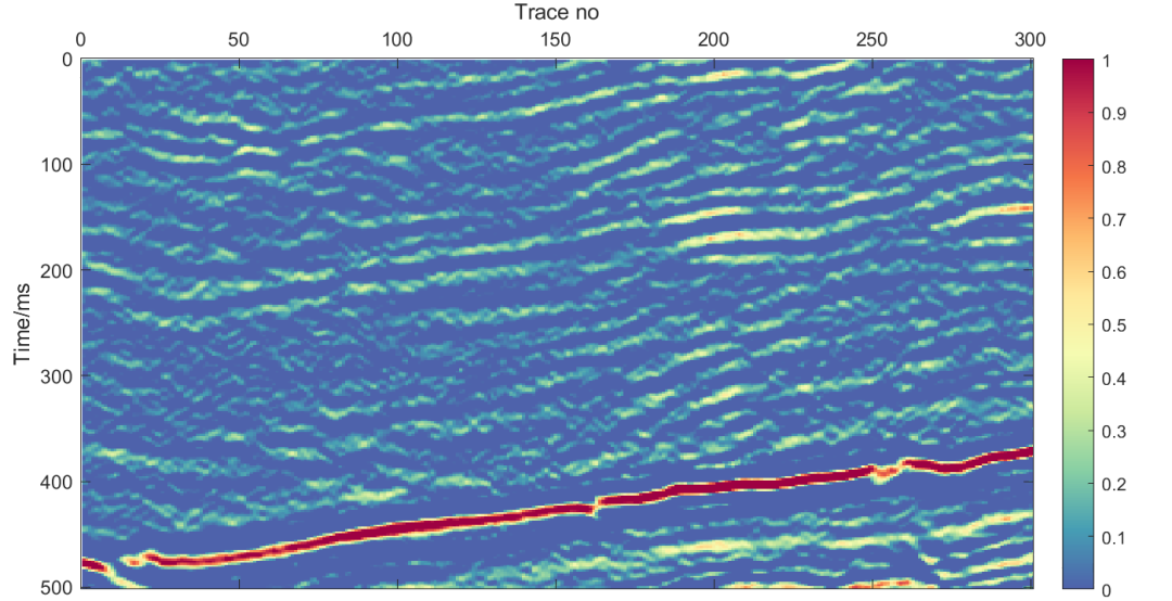 Figure 1: Pseudo-color seismic profile
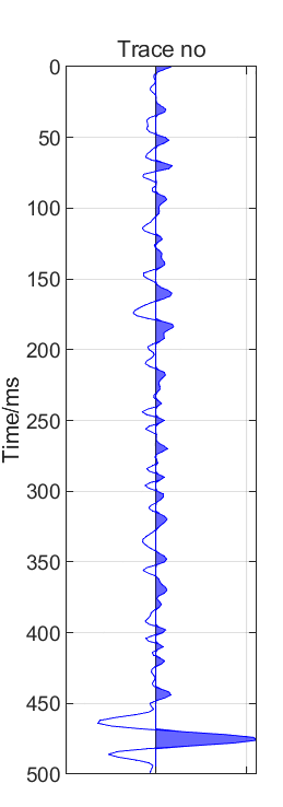
Figure 2: Single-trace record
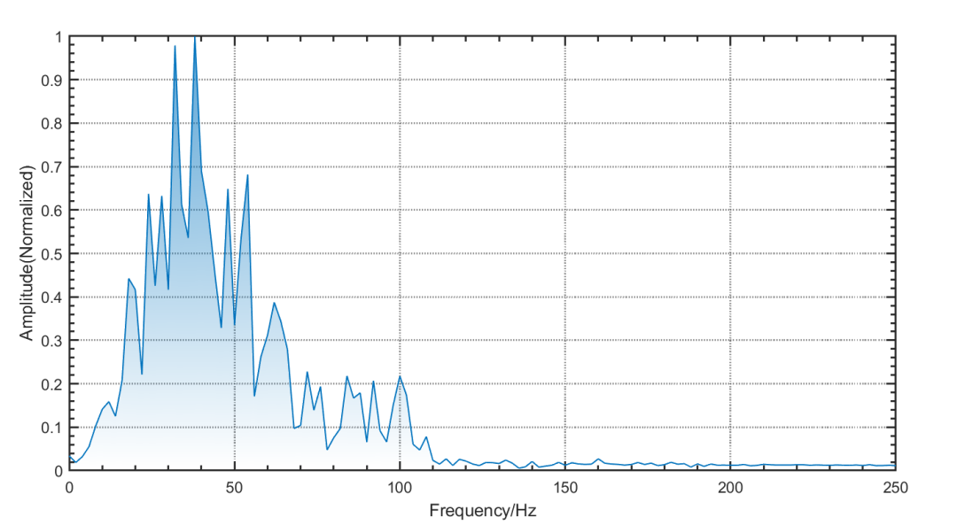 Figure 3: Seismic record spectrum
Parameters can be adjusted to change waveform color, aspect ratio, display gain, axis properties, etc.
Test data download: seismic_251_301_2ms.txt Link: https://pan.baidu.com/s/1JfKqIzG8c4s00yMwBq9reg?pwd=idip
This article has no commercial purpose, only for teaching and technical sharing. Some reference codes are provided with sources. If there is any infringement, it will be deleted immediately.
“The most needed thing in learning is not a tragic will, but a thirst for the infinite unknown.”

Text and images: Peng Zhenming
Editor: Liu SiminPreviousIssuesReview
MATLAB Image Processing | Constructing Frequency Domain Filters from Spatial Domain Templates (Complete Code Included)
MATLAB Plotting Techniques | Setting Transparency of Color Bars (Complete Code Included)
MATLAB Plotting Techniques | Capturing Frames to Generate GIF Animations (Complete Code Included)
MATLAB Plotting Techniques | Standard Labeling of Graphics (With Example Code)
MATLAB Signal Simulation | In-depth Understanding of Frequency Resolution in Fourier Transform (With Example Code)
MATLAB Image Processing | Homomorphic Filtering of Grayscale Images (Complete Code Included)
MATLAB Plotting Techniques | Drawing Dual Y-axis Line Charts (With Example Code)
MATLAB Image Processing | Sigmoid Function Contrast Stretching (With Example Code)
MATLAB Plotting Techniques | Gamma Transformation Curve of Image Grayscale (With Example Code)
MATLAB Plotting Techniques | Clever Use of Graphics Handles (With Example Code)
MATLAB Plotting Techniques | Color Filling Between Two Lines (With Source Code)
MATLAB Plotting Techniques | 3D Visualization Code Optimization of Fourier Series Expansion
MATLAB Plotting Techniques | Data Visualization Color Schemes (With Code)
MATLAB Plotting Techniques | Pseudo-coloring Grayscale Images (With Code)
MATLAB Plotting Techniques | Density Scatter Plot + Regression Line Removal (With Code)
MATLAB Plotting Techniques | 2D Scatter Plot (With Code)
MATLAB Plotting Techniques | 3D Curve Filling (With Code)
MATLAB Plotting Techniques | 3D Line Chart (With Code)
MATLAB Plotting Techniques | 3D Surface (With Code)
MATLAB Plotting Techniques | Homemade Music Player (With Code)
MATLAB Plotting Techniques | Polygon Area Filling Chart (With Code)
MATLAB Plotting Techniques | Gradient Line Chart Drawing (With Code)
MATLAB Plotting Techniques | Line Chart Drawing (With Code)
MATLAB Plotting Techniques | Gradient Bar Chart Drawing
Tell stories around you, discuss educational topics, chat about life, and write warm words.