Follow 👆 the official account and reply 'python' to receive a zero-based tutorial! Source from the internet, please delete if infringing.Introduction to Python Data Analysis Basics
1. Descriptive Statistics (descriptive statistics)
Descriptive statistics is the first step in understanding the basic characteristics of a dataset, including statistics such as mean, median, and standard deviation.
【Tutorial method to obtain at the end of the article!!】
Use the pandas library to calculate the descriptive statistics of the dataset.
import pandas as pd

# Create a dataset
data = {
    'age': [25, 30, 35, 40, 45],
    'income': [50000, 60000, 70000, 80000, 90000]
}
df = pd.DataFrame(data)

# Calculate descriptive statistics
desc_stats = df.describe()
print(desc_stats)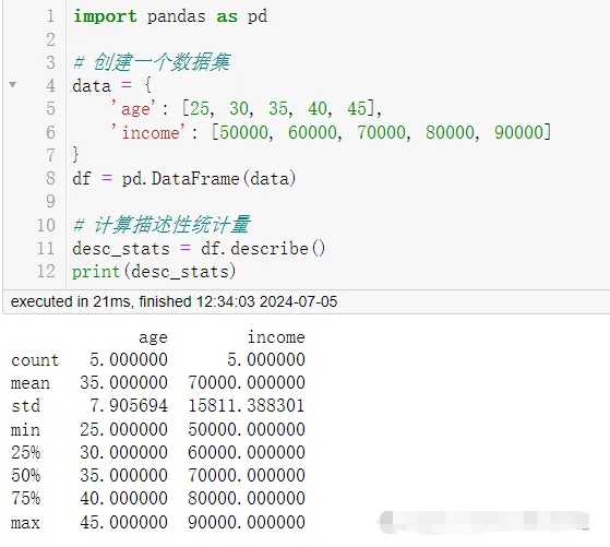
2. Data Visualization (data visualization)
Data visualization is the graphical representation of data, which helps to discover patterns, trends, and anomalies.
Use the matplotlib and seaborn libraries to create charts.
import matplotlib.pyplot as plt
import seaborn as sns

# Load built-in dataset
tips = sns.load_dataset("tips")

# Create a scatter plot
plt.figure(figsize=(10, 6))
sns.scatterplot(x="total_bill", y="tip", data=tips)
plt.title('Total Bill vs Tip')
plt.show()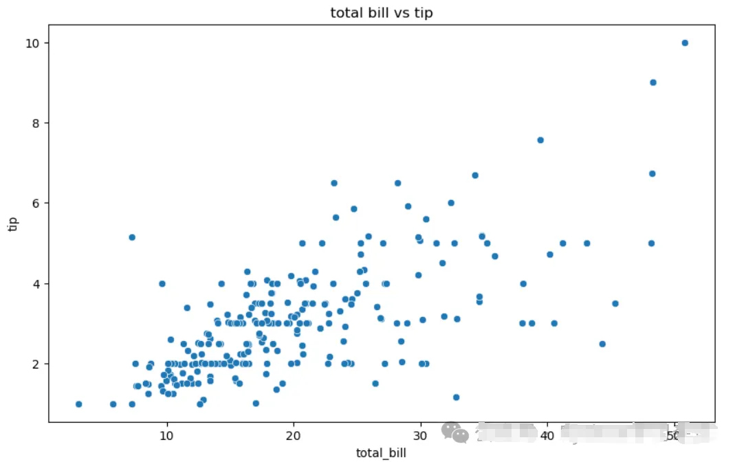

3. Exploratory Data Analysis (exploratory data analysis, EDA)
EDA is the process of understanding data using graphs and other statistical methods without explicit hypotheses.
Use pandas and matplotlib for exploratory data analysis.
# Load built-in dataset
iris = sns.load_dataset("iris")

# Use pandas to inspect data
print(iris.head())
print(iris.info())
print(iris.describe())

# Use seaborn to draw a boxplot to observe the petal length distribution of different species of iris flowers
sns.boxplot(x='species', y='petal_length', data=iris)
plt.show()
Output
   sepal_length  sepal_width  petal_length  petal_width species
0           5.1          3.5           1.4          0.2  setosa
1           4.9          3.0           1.4          0.2  setosa
2           4.7          3.2           1.3          0.2  setosa
3           4.6          3.1           1.5          0.2  setosa
4           5.0          3.6           1.4          0.2  setosa

RangeIndex: 150 entries, 0 to 149
Data columns (total 5 columns):
 #   Column        Non-Null Count  Dtype
---  ------        --------------  -----
 0   sepal_length  150 non-null    float64
 1   sepal_width   150 non-null    float64
 2   petal_length  150 non-null    float64
 3   petal_width   150 non-null    float64
 4   species       150 non-null    object
dtypes: float64(4), object(1)
memory usage: 6.0+ KB
None
       sepal_length  sepal_width  petal_length  petal_width
count    150.000000   150.000000    150.000000   150.000000
mean       5.843333     3.057333      3.758000     1.199333
std        0.828066     0.435866      1.765298     0.762238
min        4.300000     2.000000      1.000000     0.100000
25%        5.100000     2.800000      1.600000     0.300000
50%        5.800000     3.000000      4.350000     1.300000
75%        6.400000     3.300000      5.100000     1.800000
max        7.900000     4.400000      6.900000     2.500000
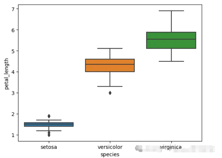
4. Hypothesis Testing (hypothesis testing)
Hypothesis testing is a statistical process to determine whether patterns in the data are caused by random variation or actual effects.
Use scipy to perform t-tests.
from scipy import stats

# Two sample datasets
group1 = [1,2,3,4,5,12,3,4,3,4,4,12,3,4,4]
group2 = [2,3,4,5,6,13,5,6,5,5,5,15,4,3,2]

# Perform independent samples t-test
t_stat, p_val = stats.ttest_ind(group1, group2)
print(f"t-statistic: {t_stat}, p-value: {p_val}")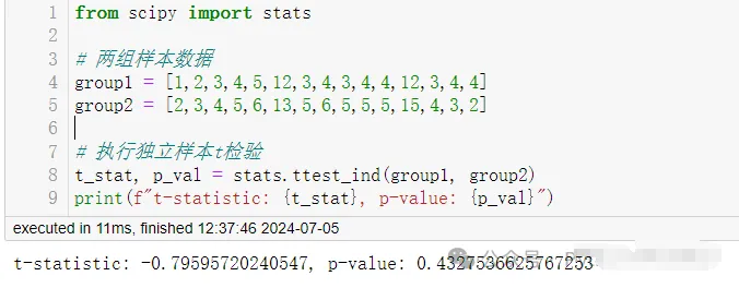
Python Deep Learning – Attention Mechanism, Transformer Models, Generative Models, Object Detection Algorithms, Graph Neural Networks, Reinforcement Learning, and Visualization Methods
Practical Tips for Python Data Analysis
Rename Columns
import pandas as pd
# Create a sample DataFrame
data = {'old_name_1': [1, 2, 3],        'old_name_2': [4, 5, 6]}
df = pd.DataFrame(data)
# Rename columns
df.rename(columns={'old_name_1': 'new_name_1', 'old_name_2': 'new_name_2'}, inplace=True)
Sometimes, you need to deal with datasets where the column names are not descriptive. You can easily rename columns using the rename method.
Filter Rows by Condition
# Filter rows where a condition is met
filtered_df = df[df['column_name'] > 3]
Filtering rows based on conditions is a common operation that allows you to select only the rows that meet specific criteria.
Handle Missing Data
# Drop rows with missing values
df.dropna()
# Fill missing values with a specific value
df.fillna(0)
Handling missing data is an important part of data analysis. You can either drop rows with missing values or fill them with default values.
Group and Summarize Data
# Group by a column and calculate mean for each group
grouped = df.groupby('group_column')['value_column'].mean()
Grouping and summarizing data is crucial for aggregating information in a dataset. You can use Pandas’ groupby method to calculate statistics for each group.
Pivot Tables
# Create a pivot table
pivot_table = df.pivot_table(values='value_column', index='row_column', columns='column_column', aggfunc='mean')
Pivot tables help reshape data and summarize it in tabular form. They are especially useful for creating summary reports.
Merge DataFrames
# Merge two DataFrames
merged_df = pd.merge(df1, df2, on='common_column', how='inner')
When you have multiple datasets, you can merge them based on common columns using Pandas’ merge function.
Apply Custom Functions
# Apply a custom function to a column
def custom_function(x):    return x * 2
df['new_column'] = df['old_column'].apply(custom_function)
You can apply custom functions to columns, which is particularly useful when you need to perform complex transformations.

Resample Time Series Data
# Resample time series data
df['date_column'] = pd.to_datetime(df['date_column'])
df.resample('D', on='date_column').mean()
When dealing with time series data, Pandas allows you to resample data to different time frequencies, such as daily, monthly, or yearly.
Handle Categorical Data
# Convert categorical data to numerical using one-hot encoding
df = pd.get_dummies(df, columns=['categorical_column'])
Categorical data often needs to be converted to numerical form for use in machine learning models. One common method is one-hot encoding.
Export Data
# Export DataFrame to CSV
df.to_csv('output.csv', index=False)
One-Liner List Definition
When defining a certain list, writing a for loop can be cumbersome. Fortunately, Python has a built-in method that can solve this problem in one line of code. Below is a comparison of creating a list using a for loop and creating a list in one line of code.
x = [1,2,3,4]
out = []
for item in x:
  out.append(item**2)
print(out)

[1, 4, 9, 16]

# vs.

x = [1,2,3,4]
out = [item**2 for item in x]
print(out)

[1, 4, 9, 16]
Lambda Expressions
Are you tired of defining functions that you only use a few times? Lambda expressions are your savior! Lambda expressions are used to create small, one-time, and anonymous function objects in Python, which can create a function for you.
The basic syntax of a lambda expression is:
lambda arguments: expressionlambda arguments: expression
Note! As long as there is a lambda expression, it can perform any operation that a regular function can execute.
You can feel the powerful functionality of lambda expressions from the following example:
double = lambda x: x * 2
print(double(5))

10
Map and Filter
Once you master lambda expressions, learning to combine them with the Map and Filter functions can achieve even more powerful functionality. Specifically, map transforms each element in the list by performing some operation and converts it into a new list.
In this example, it iterates through each element and multiplies it by 2, forming a new list. (Note! The list() function simply converts the output to list type)
# Map
seq = [1, 2, 3, 4, 5]
result = list(map(lambda var: var*2, seq))
print(result)

[2, 4, 6, 8, 10]
The Filter function takes a list and a rule, similar to map, but it returns a subset of the original list by comparing each element with the Boolean filtering rule.
# Filter
seq = [1, 2, 3, 4, 5]
result = list(filter(lambda x: x > 2, seq))
print(result)

[3, 4, 5]
Arange and Linspace
Arange returns an arithmetic list with a given step size. Its three parameters start, stop, and step represent the starting value, ending value, and step size, respectively. Note! The stop point is a