Spherical Harmonics and Helmholtz Decomposition in Atmospheric Modeling

Skyborn

When dealing with global circulation, a ghostly problem always haunts us—the Pole Problem. On the latitude-longitude grid, all meridians converge at the poles, leading to severe distortion of grid cells, which not only brings great trouble to calculations (CFL condition), but may also introduce unrealistic errors.

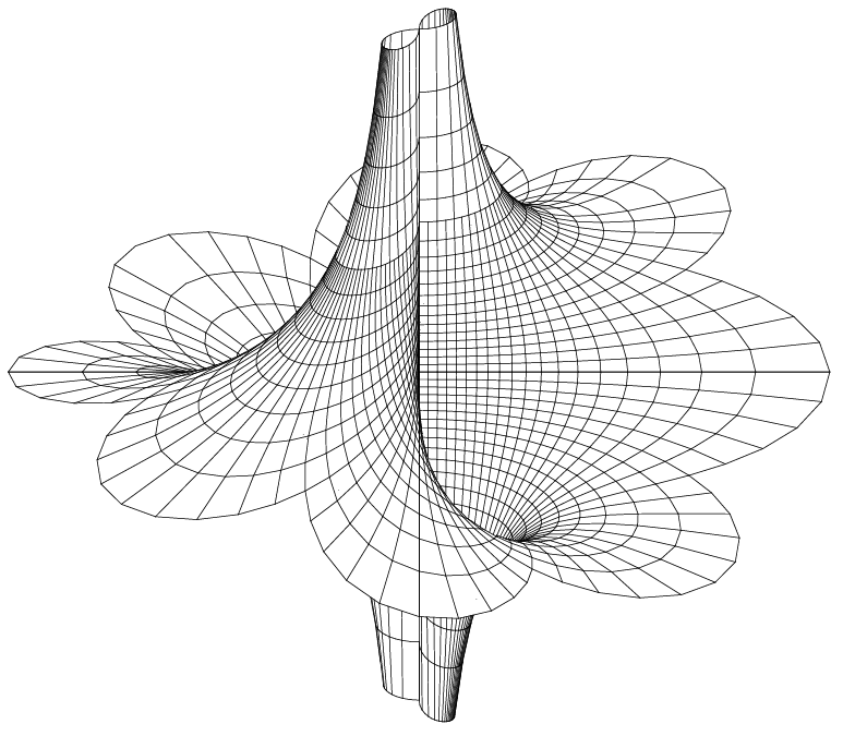
So, is there a more natural and elegant way to describe our rotating sphere?

The answer is yes. Today, we will discuss the beautiful mathematical tool behind atmospheric models—spherical harmonics.

First Movement: Spherical Harmonics—The “Notes” Composed for Earth

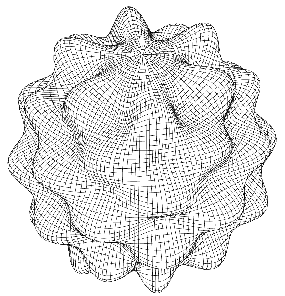
Imagine that any complex sound wave can be decomposed into a series of simple sine waves (fundamental frequency, harmonics…). Similarly, any scalar field defined on the sphere (such as temperature, pressure, or potential height) can also be decomposed into a set of standard, orthogonal “basis shapes”.

These “basis shapes” are the spherical harmonics.

In the ECMWF IFS model, a physical quantity A at a specific time t and vertical level η is represented by a truncated series of spherical harmonics:

This formula is the core of the spectral model! Let’s break it down:

: The value of the physical quantity at the grid point (e.g., temperature, potential). Here, is longitude, is latitude.
: This is the complex spectral coefficient that we are really concerned about. It is what the model forecasts and stores.
: The normalized associated Legendre polynomials, which describe the structure of the physical quantity in the north-south direction.
:Fourier functions (sine/cosine waves in complex exponential form), which describe the structure of the physical quantity in the east-west direction.
and : These are the two key integers that determine the shape of the spherical harmonics, known as total wavenumber and zonal wavenumber.

❝

Order n (Total Wavenumber): The total wavenumber determines the overall complexity of the harmonics in both directions. The larger the n, the smaller and more detailed the spatial scale of phenomena that can be described.

Degree m (Zonal Wavenumber): The zonal wavenumber determines how many waves the harmonics have in the east-west direction. Physically, it must satisfy .

The great advantage of spherical harmonics is:

Globality and Orthogonality: They are functions defined over the entire sphere, naturally avoiding the pole problem.
Scale Separation: It transforms the physical field from the “spatial domain” to the “wavenumber domain”, allowing us to clearly analyze the contributions of systems at different scales (such as planetary waves, weather-scale systems).

Triangular Truncation in Spectral Space

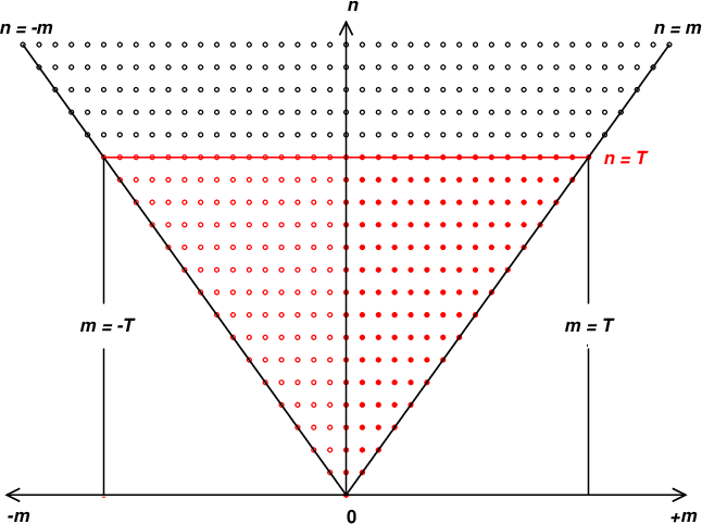
Theoretically, n can take on an infinite value. However, in numerical models, we must make trade-offs and only retain the most important parts. The model sets a maximum total wavenumber T, and all harmonics with n > T are discarded. This process is called triangular truncation.

This T value directly defines the model’s horizontal resolution. The ECMWF resolutions we often hear about, T639 and T1279, refer to T=639 and T=1279.

The following figure clearly shows the wavenumber space of spherical harmonics (n, m) and triangular truncation:

❝

It can be said that spherical harmonics are the “musical score” for describing the Earth’s physical fields.

Second Movement: Helmholtz Decomposition—Analyzing the “Soul” of Wind Fields 💨

Spherical harmonics perfectly solve scalar fields. But what about the wind field, which is a vector field? What should we do?

Here we introduce another powerful mathematical tool—Helmholtz Decomposition.

The core idea is:Any global wind field can be uniquely decomposed into two parts:

Rotational Wind Component (Rotational/Non-divergent): This part can be described by a scalar stream function (). It represents the rotational component of the wind field, which we usually refer to as vorticity. Most of the kinetic energy on Earth is concentrated in this part, such as cyclones, anticyclones, and other large vortex systems.
Divergent Wind Component (Divergent/Irrotational): This part is described by a scalar velocity potential (). It represents the divergence/convergence of the wind field, closely related to vertical motion, precipitation, energy conversion, and other key weather processes.

In other words, any global wind field can be uniquely decomposed into the superposition of these two parts:

where is related to , and is related to .

The significance of this decomposition is that it breaks down the complex vector wind field into two scalar fields (stream function and velocity potential) with clear physical meanings!

Why is Global Decomposition the Most Accurate?

1. Global Closed System does not have the “artificial boundary conditions” that regional atmospheric models hate; all calculations are completed within a self-consistent mathematical framework, ensuring the conservation of energy and vorticity, making it the theoretically most accurate global analysis method.

2. Avoiding Pole Singularity Geometric distortions can lead to catastrophic consequences mathematically. Even for smooth wind fields, certain derivatives can tend to infinity at the poles, causing traditional finite difference methods to fail completely at the poles. Spherical harmonic decomposition fundamentally bypasses this “coordinate singularity”.

3. Accurate Scale Separation

Large Scale (n=1-10): Planetary waves, jet streams
Weather Scale (n=20-100): Cyclones, anticyclones
Small Scale (n>100): Mesoscale convection, turbulence

Characteristics	Limited Area Model	Global Model
Boundary	There are artificial, open boundaries	No boundaries, it is a closed system
Boundary Conditions	Must be specified artificially, introducing huge errors	Natural periodicity, determined by the data itself
Accuracy	Severely “polluted” by boundary assumptions, lower precision	Theoretically most accurate, avoiding boundary errors
Physical Consistency	Energy and vorticity may “leak” at the boundaries, not conserved	Global conservation of energy and vorticity, more realistic physical processes

Third Movement: Perfect Harmony—When Spherical Harmonics Meet Helmholtz Decomposition

Now, how do we combine these two?

The answer is: Use spherical harmonics to expand the stream function and velocity potential!

This is the core step of the Global Spectral Model:

Analysis: Starting from the wind field on the grid, calculate the global vorticity and divergence.
Spectral Transformation: Both vorticity and divergence are scalar fields! We can expand them using spherical harmonics to obtain their spectral coefficients in the “wavenumber domain” and .
Solving: In the wavenumber domain, solving the complex Poisson equations for the stream function and velocity potential becomes extremely simple algebraic operations:
Synthesis: With the spectral coefficients of and , we can reverse synthesize the rotational and divergent wind components at any point globally, thus reconstructing the complete wind field. The uv2dvf in NCL is also based on this idea.

Cornerstone: SPHEREPACK

The theory is so beautiful, but implementing it requires solid computational tools. As early as the 1970s to 1990s, Paul Noble Swarztrauber at the National Center for Atmospheric Research (NCAR) led the development of a software package specifically for harmonic analysis on the sphere—SPHEREPACK.

SPHEREPACK is an efficient and reliable library of subroutines written in FORTRAN, containing tools to implement all the “magic” mentioned above:

Although there are many more modern languages and tools now, SPHEREPACK remains the cornerstone of many weather and climate model dynamics.

As we enjoy the convenience brought by high-resolution models today, we should not forget pioneers like Paul Noble Swarztrauber.

Modern Revolution: From SPHEREPACK to Skyborn

However, with the rise of Python in the field of scientific computing, traditional SPHEREPACK faces new challenges:

The “Nightmare” of Traditional Installation:

# Traditional windspharm installation process (painful)
1. Download SPHEREPACK Fortran source code
2. Configure a complex compilation environment
3. Handle various platform compatibility issues
4. Debug compilation errors...

Skyborn’s One-Click Solution:

# Now it only takes (simple)
pip install skyborn

It’s that simple!

Precompiled all Fortran extensions: Cross-platform compatibility, no local compilation required (supports Linux, Windows, Intel MacOS 13+, Apple silicon MacOS 14+)
Modernized Fortran: Traditional Fortran77 code has been optimized to modern Fortran
Maintaining Performance Advantages: Based on the efficient core of NCAR SPHEREPACK, consistent with the computational ideas in NCL.

Skyborn.windspharm: Practice

Now, let’s see how these beautiful theories are easily implemented in Skyborn:

from skyborn.windspharm.standard import VectorWind
import numpy as np

# Load global wind field data (supports various grids)
nlat, nlon = 73, 144# T42 resolution
u = load_zonal_wind_data()      # Zonal wind component
v = load_meridional_wind_data() # Meridional wind component

# Initialize spherical harmonics analyzer
vw = VectorWind(u, v, gridtype='gaussian')  # Supports Gaussian grid

# Perform Helmholtz decomposition
psi, chi = vw.sfvp()                        # Stream function and velocity potential
vorticity = vw.vorticity()                  # Relative vorticity
divergence = vw.divergence()                # Horizontal divergence

# Complete decomposition analysis
u_rot, v_rot, u_div, v_div = vw.helmholtz() # Rotational and divergent wind components

# Advanced diagnostic quantities
rws = vw.rossbywavesource()                 # Rossby wave source
abs_vort = vw.absolutevorticity()           # Absolute vorticity
rws = vw.rossbywavesource()                 # Calculate Rossby wave source

These few lines of code achieve the complete process from SPHEREPACK to global spectral analysis.

Note: You need to provide global data without missing values; if there are missing values, refer to the previous post: Python | Skyborn | Missing Value Filling

Skyborn Computational Results Display

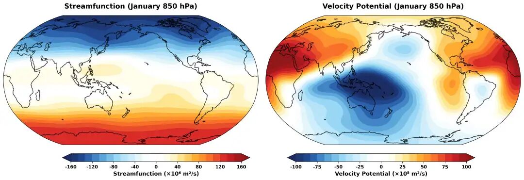
Stream Function and Velocity Potential

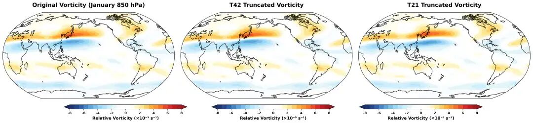
Different Triangular Truncations

Rossby Wave Source

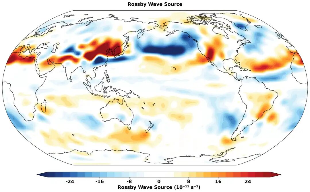
The calculation method is consistent with the previous post: NCL | Rossby Wave Source | Rossby Wave Source

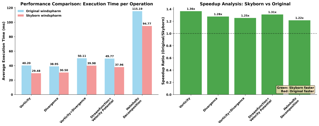
Benchmark Testing

❝

For more information and code due to the length of the code, please visit: Skyborn documentation———https://skyborn.readthedocs.io/en/latest/

Conclusion: From Theory to Practice

From the annoying pole problem, to the beautiful spherical harmonics, then to the profound Helmholtz decomposition, and finally landing on the modernized Skyborn tool—this is a complete evolution from mathematical theory to engineering practice.

SPHEREPACK laid a solid theoretical foundation for us, carrying half a century of numerical computation wisdom. Meanwhile, Skyborn builds on this foundation, modernizing these powerful tools to make them accessible to everyone.

When you see those smooth and flowing global circulation animations, remember:

Behind them echoes a mathematical symphony composed of countless “spherical harmonics”
Now you only need one line of code pip install skyborn to conduct this perfect concerto of nature and mathematics

Reference

https://skyborn.readthedocs.io/en/latest/index.html
Swarztrauber, P. N. (2003), “On computing the points and weights for Gauss–Legendre quadrature”, SIAM Journal on Scientific Computing, 24(3), 945–954.
Swarztrauber, P. N., and W. F. Spotz (2000), “Generalized discrete spherical harmonic transforms”, Journal of Computational Physics, 159(2), 213–230.
Adams, J. C., and P. N. Swarztrauber (1999), “SPHEREPACK 3.0: A model development facility”, Monthly Weather Review, 127(8), 1872–1878.
Swarztrauber, P. N. (1996), “Spectral transform methods for solving the shallow-water equations on the sphere”, Monthly Weather Review, 124(4), 730–744.
Williamson, D. L., et al. (1992), “A standard test set for numerical approximations to the shallow water equations in spherical geometry”, Journal of Computational Physics, 102(1), 211–224.
https://confluence.ecmwf.int/
https://github.com/ajdawson/windspharm
https://github.com/jswhit/pyspharm
https://www.chicagotribune.com/obituaries/paul-swarztrauber-longmont-co/
https://www.findagrave.com/memorial/75142880/paul_noble-swarztrauber