
Many people often use simple linear regression when doing data analysis, which is the simplest regression model to describe the statistical relationship between two variables. However, in real-world problems, we often encounter linear relationships among multiple variables, which requires the use of multiple linear regression. Multiple linear regression is a generalization of simple regression and is widely used in practical applications. This article will demonstrate how to use Python code to solve practical problems using multiple linear regression.
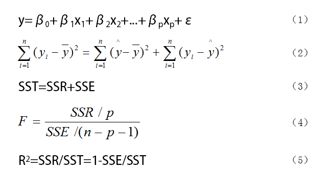
Figure 1. The formula used in the multiple regression model
As shown in Figure 1, we assume that the linear regression model between the random variable y and the general variables x1, x2, ..., xp is expressed as (1), where y is the dependent variable, x1, x2, ..., xp are the independent variables, β1, β2, ..., βp are the regression coefficients, and β0 is the regression constant. For a practical problem, if we obtain n sets of observational data (xi1, xi2, ..., xip; y) (i = 1, 2, ..., n), we can write these n sets of observational data in matrix form y = Xβ + ε.
After obtaining the regression equation, we often need to perform significance tests on the regression equation. The significance test here mainly includes three parts. The first is the F-test, which tests whether the independent variables x1, x2, ..., xp have a significant impact on y as a whole, mainly using equations (2), (3), and (4), where (2) and (3) are the same equation expressed with different symbols; the second is the t test, which conducts significance tests for each independent variable to see whether each independent variable has a significant effect on y, which is different from the overall test; the third is the goodness of fit, which is R2, whose value ranges from 0 to 1; the closer it is to 1, the better the regression fit, and the closer to 0, the worse the effect. However, R can only intuitively reflect the fitting effect and cannot replace F test as a strict significance test.
The above is a simple introduction to multiple linear regression. The detailed principles are extensive, and interested readers can refer to relevant literature. Here, we will focus on how to analyze using Python. Next, we will use code to demonstrate the analysis process of multiple linear regression.
The data we use comes from the 2013 “China Statistical Yearbook”, where the residents’ consumption expenditure is the dependent variable y, and the other 9 variables are independent variables. Among them, x1 is the food expenditure of residents, x2 is the clothing expenditure, x3 is the housing expenditure, x4 is the healthcare expenditure, x5 is the cultural and entertainment expenditure, x6 is the average salary of employees, x7 is the per capita GDP of the region, x8 is the regional consumer price index, and x9 is the regional unemployment rate. In all these variables, x1 to x7 and y are in yuan, x9 is in percentage, and x8 has no unit because it is a consumer price index. The overall size of the data is 31×10, that is, 31 rows and 10 columns, as shown in Figure 2.
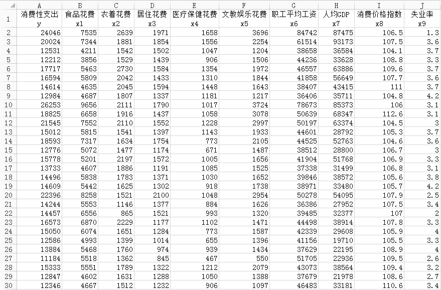
Figure 2. Partial content of the dataset
First, we need to import the necessary libraries.
import numpy as np
import pandas as pd
import statsmodels.api as sm
Next is data preprocessing. Since the original data’s column names are too long, we need to process them by removing the Chinese characters and keeping only the English names.
file = r'C:\Users\data.xlsx'
data = pd.read_excel(file)
data.columns = ['y', 'x1', 'x2', 'x3', 'x4', 'x5', 'x6', 'x7', 'x8', 'x9']
Then we start generating the multiple linear model, as shown in the code below.
x = sm.add_constant(data.iloc[:,1:]) # Generate independent variables
y = data['y'] # Generate dependent variable
model = sm.OLS(y, x) # Generate model
result = model.fit() # Model fitting
result.summary() # Model summary
It is clear that the independent variables refer to x1 to x9, and the code data.iloc[:,1:] removes the first column of the original data, which is the data for y. The result.summary() generates a result summary, as shown in Figure 3.
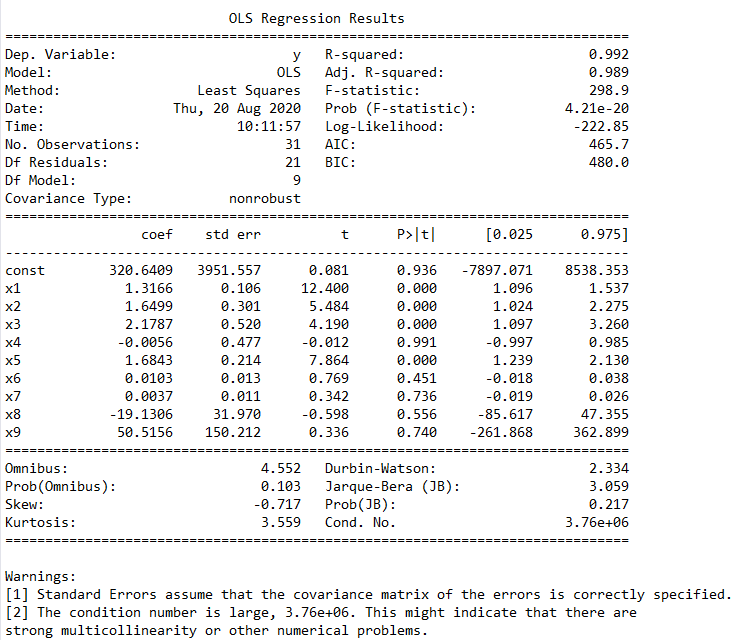
Figure 3. Regression results including all independent variables
In this result, we mainly look at the columns "coef", "t", and "P>|t|". coef is the regression coefficient mentioned earlier, and the value of const is the regression constant. Therefore, the regression model we obtain is y = 320.640948 + 1.316588 x1 + 1.649859 x2 + 2.17866 x3 - 0.005609 x4 + 1.684283 x5 + 0.01032 x6 + 0.003655 x7 -19.130576 x8 + 50.515575 x9. The columns "t" and "P>|t|" are equivalent; you can choose one of them for use, and they are mainly used to determine the linear significant relationship of each independent variable with y, which we will discuss later. From the figure, we can also see that Prob (F-statistic) is 4.21e-20, which is the commonly used P-value close to zero, indicating that our multiple linear equation is significant, meaning that y has a significant linear relationship with x1, x2, ..., x9, and R-squared is 0.992, which also indicates that this linear relationship is quite significant. Theoretically, this multiple linear equation has been derived, and the effect is good, so we can use it for prediction. However, we still need to explore further. As mentioned earlier, y has a significant linear relationship with x1, x2, ..., x9, but note that x1 to x9 are considered as a whole. This does not mean that y has a significant linear relationship with each independent variable. We need to identify those independent variables that do not have a significant linear relationship with y and remove them, leaving only those that are significantly related. This is the t test mentioned earlier. The principle of the t test is somewhat complex, and interested readers can refer to the materials themselves. Here, we will not elaborate further. We can use the "P>|t|" column in Figure 3 to determine this. In this column, we can set a threshold, such as 0.05, 0.02, or 0.01, which are commonly used in statistics. We will use 0.05 here; any independent variable with P>|t| greater than 0.05 will be removed. These are the independent variables that do not have a significant linear relationship with y, so they will be discarded. Please note that the independent variables refer to x1 to x9, excluding the value of const in Figure 3. However, there is a principle that only one can be removed at a time, and the one removed is usually the one with the largest P-value. For example, in Figure 3, the largest P-value is x4, so it will be removed, and then we will repeat the modeling process with the remaining x1, x2, x3, x5, x6, x7, x8, x9, and find the one with the largest P-value to remove. This process is repeated until all P-values are less than or equal to 0.05. The remaining independent variables are the ones we need, and all these independent variables have a significant linear relationship with y. We will use these independent variables for modeling.
We can write the above process into a function named looper, as shown in the code below.
def looper(limit):
    cols = ['x1', 'x2', 'x3', 'x5', 'x6', 'x7', 'x8', 'x9']
    for i in range(len(cols)):
        data1 = data[cols]
        x = sm.add_constant(data1) # Generate independent variables
        y = data['y'] # Generate dependent variable
        model = sm.OLS(y, x) # Generate model
        result = model.fit() # Model fitting
        pvalues = result.pvalues # Get all P-values from the results
        pvalues.drop('const', inplace=True) # Remove const
        pmax = max(pvalues) # Select the maximum P-value
        if pmax > limit:
            ind = pvalues.idxmax() # Find the index of the maximum P-value
            cols.remove(ind) # Remove this index from cols
        else:
            return result

result = looper(0.05)
result.summary()
The results are shown in Figure 4. From the results, we can see that the remaining effective variables are x1, x2, x3, and x5, and the multiple linear model we obtain is y = -1694.6269 + 1.3642 x1 + 1.7679 x2 + 2.2894 x3 + 1.7424 x5, which is the effective multiple linear model we will use.
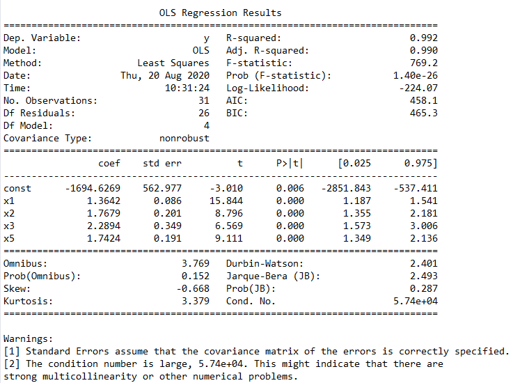
Figure 4. Regression model after removing ineffective variables
Now the question arises: which model should we choose, the first model that includes all independent variables or this model after removing some variables? After all, the overall linear effect of the first model is quite significant. Based on my experience, it still depends on the specific project requirements. The problems we encounter in practical projects are real-life examples, not just pure mathematical problems. For example, in this case, the consumer price index x8 and the unemployment rate x9 certainly have some impact on y. Blindly removing them may adversely affect the final results. Therefore, we should make decisions based on actual needs.
Finally, there is another issue to discuss: in this example, we did not standardize the original data. Should we standardize the original data in data analysis?
This also depends on the situation. In this case, the data has specific dimensions and units, so there is no need to standardize it. The linear regression model we obtain is based on the original variables, and this equation contains physical units, which means they have certain practical significance. In this case, by inputting specific values of independent variables, we can obtain the corresponding y value, and the prediction effect is straightforward. This is the benefit of performing linear fitting on original data.
If we standardized the original data, the situation would be different. After standardization, the physical units of the independent and dependent variables are lost. It would be very troublesome to make predictions with this model. We would need to standardize the new independent variable values, and the resulting y would still be standardized data, making it difficult to see its actual size and physical significance. Of course, for some purely mathematical problems where the variables have no units, standardization can be beneficial for problem analysis. So this still depends on the situation.
For the source code and data download method, please see the end of the article. To discuss the content of this article, you can add “Python Assistant” at the end of the article to join the WeChat group for communication!
Author’s Introduction: Mort, a data analysis enthusiast, specializes in data visualization and is particularly interested in the field of machine learning. I hope to learn and communicate more with friends in the industry.
Appreciate the author

The Python Chinese Community, as a decentralized global technical community, aims to become the spiritual tribe of 200,000 Chinese Python developers worldwide. It currently covers major mainstream media and collaboration platforms and has established extensive contacts with well-known companies and technical communities such as Alibaba, Tencent, Baidu, Microsoft, Amazon, Open Source China, CSDN, etc. It has tens of thousands of registered members from more than a dozen countries and regions, representing government agencies, research institutions, financial institutions, and well-known companies at home and abroad, such as the Ministry of Industry and Information Technology, Tsinghua University, Peking University, Beijing University of Posts and Telecommunications, People’s Bank of China, Chinese Academy of Sciences, China International Capital Corporation, Huawei, BAT, Google, Microsoft, etc. Nearly 200,000 developers across the entire platform are following.
Long press to scan the code to add “Python Assistant”
Then reply“Multiple” to obtain the source code data of this article

▼Click to become a community member. If you like it, please give it a thumbs up and take a look