
Source: DeepHub IMBA

This article is approximately 5000 words long and is recommended to be read in 5 minutes.
This article compares six of the most commonly used causal inference libraries in the community: <strong>Bnlearn, Pgmpy, CausalNex, DoWhy, PyAgrum, and CausalImpact</strong>.
In the Python ecosystem, there are many causal libraries to choose from, and the choice often depends on your understanding of the model and the project’s requirements for “explainability”. This article compares six of the most commonly used causal inference libraries: Bnlearn, Pgmpy, CausalNex, DoWhy, PyAgrum, and CausalImpact.
Bayesian Causal Models
In causal inference, all variables can be roughly divided into two types:driver variables and passenger variables.Driver variables directly affect the outcome, while passenger variables are related to the outcome but do not directly influence it. Distinguishing between these two is key to the entire causal analysis. For example, in predictive maintenance or equipment failure analysis, if we can identify the few variables that “cause failures”, subsequent monitoring and optimization strategies can be targeted.
Sometimes, seemingly unrelated variables actually hide important effects. For instance, suppose the engine failure rate in a factory varies greatly across different regions; you might think this is due to geographical differences, but the real cause could be latent driver factors such as humidity, maintenance cycles, or personnel experience within the factory. The value of causal inference lies here—it helps distinguish between “apparent correlations” and “true causes”.
Compared to pure predictive models, causal inference is more about answering “why” rather than “how much”. By identifying the variables that truly matter in the system, we can explain the model’s behavior and make effective interventions in the system.
Dataset and Overall Experimental Approach
To make the comparison more intuitive, all experiments used the same dataset:Census Income dataset. This classic dataset contains 48,842 records and 14 variables, most of which are discrete features. The goal is simple: Does having a postgraduate degree significantly increase the probability of earning over $50K annually?
The following code is used to load and clean the data. Continuous variables and sensitive features (such as gender, race, etc.) are removed to focus on the causal structure learning of discrete features.
# Install
pip install datazets

# Import libraries
import datazets as dz
import pandas as pd
import numpy as np
import matplotlib.pyplot as plt

# Import dataset and remove continuous and sensitive features
df = dz.import_example(data='census_income')

# Data cleaning
drop_cols = ['age', 'fnlwgt', 'education-num', 'capital-gain', 'capital-loss', 'hours-per-week', 'race', 'sex']
df.drop(labels=drop_cols, axis=1, inplace=True)

# Print sample
df.head()
1. Bnlearn
<span><span>bnlearn</span></span> is a highly encapsulated Bayesian network library that integrates almost all standard processes of causal analysis into a single API. It supports discrete, continuous, and mixed-type data, and can perform structure learning, parameter learning (CPD estimation), inference and synthetic data generation. More importantly, it provides commonly used independence tests, scoring functions, topological sorting, model comparison, and visualization as ready-to-use functions.
Below is the complete code for learning the structure using HillClimbSearch and BIC scoring method.
# Install
pip install bnlearn
# Load library
import bnlearn as bn
# Structure learning
model = bn.structure_learning.fit(df, methodtype='hillclimbsearch', scoretype='bic')
# Test edge significance and prune
model = bn.independence_test(model, df, test="chi_square", alpha=0.05, prune=True)
# Parameter learning (optional)
model = bn.parameter_learning.fit(model, df)
# Plot graph
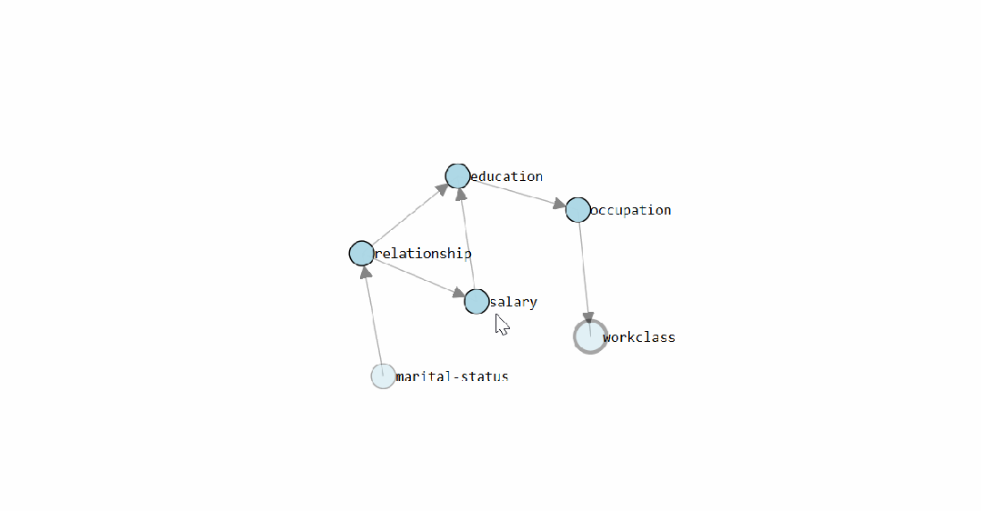
G = bn.plot(model, interactive=False)
dotgraph = bn.plot_graphviz(model)
dotgraph.view(filename=r'c:/temp/bnlearn_plot')The learned DAG (Directed Acyclic Graph) structure of the model is as follows:
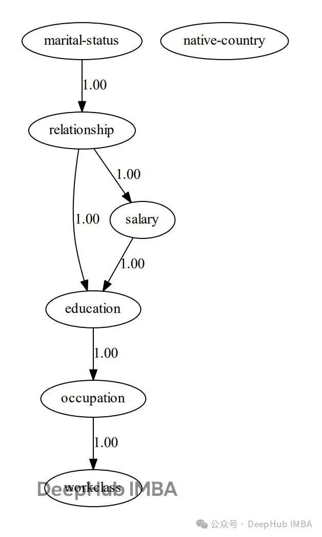
The static graph shows the causal structure graph learned by <span><span>bnlearn</span></span> for the Census Income dataset. The interactive version allows direct viewing of the conditional probability distribution for each edge.
After the DAG is learned, inference can be performed directly. For example, calculating the posterior probability of earning over $50K when the education level is a doctorate:
# Start inference
query = bn.inference.fit(model, variables=['salary'], evidence={'education':'Doctorate'})
print(query)
The results are as follows:
salary <=50K : 29.1%
salary >50K  : 70.9%
This probability aligns with our understanding: a doctoral degree indeed leads to a higher income range.
Now let’s try again with a high school graduate (<span><span>HS-grad</span></span>) :
query = bn.inference.fit(model, variables=['salary'], evidence={'education':'HS-grad'})The result is:
salary <=50K : 83.8%
salary >50K  : 16.2%
We can also combine multiple conditions, for example:
# When education=Doctorate and marital-status=Never-married, predict workclass
query = bn.inference.fit(model, variables=['workclass'], evidence={'education':'Doctorate', 'marital-status':'Never-married'})
Overall, <span><span>bnlearn</span></span> is suitable for quickly building causal structures and performing probabilistic inference, with complete functionality. Input data can be discrete, continuous, or mixed types. For those who want to quickly validate causal hypotheses in business scenarios, this library has a very gentle learning curve.
2. Pgmpy
<span><span>Pgmpy</span></span> is a more low-level probabilistic graphical model library. If <span><span>bnlearn</span></span> is “out-of-the-box”, then <span><span>pgmpy</span></span> is more like a “toolbox”. Its flexibility is very high, but it also means that a strong foundation in Bayesian modeling is required.
These two libraries have overlapping functionalities because <span><span>bnlearn</span></span> relies on <span><span>pgmpy</span></span> for its underlying implementation. However, in <span><span>pgmpy</span></span>, all steps must be built manually: data processing, modeling, parameter estimation, inference, and visualization must all be written by the user.
Below is an example of structure learning using <span><span>HillClimbSearch</span></span> and <span><span>BIC</span></span> scoring method:
# Install pgmpy
pip install pgmpy

# Import functions
from pgmpy.estimators import HillClimbSearch, BicScore, BayesianEstimator
from pgmpy.models import BayesianNetwork, NaiveBayes
from pgmpy.inference import VariableElimination

# Import data and remove continuous and sensitive features
df = bn.import_example(data='census_income')
drop_cols = ['age', 'fnlwgt', 'education-num', 'capital-gain', 'capital-loss', 'hours-per-week', 'race', 'sex']
df.drop(labels=drop_cols, axis=1, inplace=True)

# Create estimator and scoring method
est = HillClimbSearch(df)
scoring_method = BicScore(df)

# Build model and print edges
model = est.estimate(scoring_method=scoring_method)
print(model.edges())
After building the structure, you need to manually fit the conditional probability distributions (CPD):
vec = {
    'source': ['education', 'marital-status', 'occupation', 'relationship', 'relationship', 'salary'],
    'target': ['occupation', 'relationship', 'workclass', 'education', 'salary', 'education'],
    'weight': [True, True, True, True, True, True]
}
vec = pd.DataFrame(vec)

# Create Bayesian model
bayesianmodel = BayesianNetwork(vec)

# Fit model
bayesianmodel.fit(df, estimator=BayesianEstimator, prior_type='bdeu', equivalent_sample_size=1000)

# Inference
model_infer = VariableElimination(bayesianmodel)
query = model_infer.query(variables=['salary'], evidence={'education':'Doctorate'})
print(query)
The output results are basically consistent with those from <span><span>bnlearn</span></span>:
 salary <=50K : 29.1%
 salary >50K  : 70.9%
The difference is that this process requires you to define the DAG, parameter estimation, and inference methods yourself. This library is highly flexible but is clearly more suitable for researchers or developers creating custom causal frameworks, rather than business personnel who want to “get started quickly”.
3. CausalNex
<span><span>CausalNex</span></span> is a Python library focused on learning causal graphs from data and quantifying causal effects. It only supports discrete distributions, which is important. Therefore, all continuous variables or high cardinality features must be discretized before modeling, otherwise the model cannot fit.
The documentation also clearly states that if there are too many features or complex states, the model’s performance will significantly decline. However, the advantage is that it provides some convenient functions to help reduce the number of categories and handle label encoding.
Below is a complete example, still using the same Census Income data. The first step is to convert all categorical variables to numeric (because the NOTEARS algorithm requires matrix calculations):
# Install
pip install causalnex

# Import libraries
from causalnex.structure.notears import from_pandas
from causalnex.network import BayesianNetwork
import networkx as nx
import datazets as dz
from sklearn.preprocessing import LabelEncoder
import matplotlib.pyplot as plt
le = LabelEncoder()

# Import data and remove continuous and sensitive features
df = dz.get(data='census_income')

drop_cols = ['age', 'fnlwgt', 'education-num', 'capital-gain', 'capital-loss', 'hours-per-week', 'race', 'sex']
df.drop(labels=drop_cols, axis=1, inplace=True)

# Convert to numeric
df_num = df.copy()
for col in df_num.columns:
    df_num[col] = le.fit_transform(df_num[col])
The structure learning part uses the NOTEARS algorithm, which can automatically derive the DAG from the correlation matrix. However, the output may be too dense, so a threshold must be set to filter out weak edges:
# Structure learning
sm = from_pandas(df_num)

# Threshold pruning
sm.remove_edges_below_threshold(0.8)

# Plotting
plt.figure(figsize=(15,10))
edge_width = [d['weight']*0.3 for (u,v,d) in sm.edges(data=True)]
nx.draw_networkx(sm, node_size=400, arrowsize=20, alpha=0.6, edge_color='b', width=edge_width)
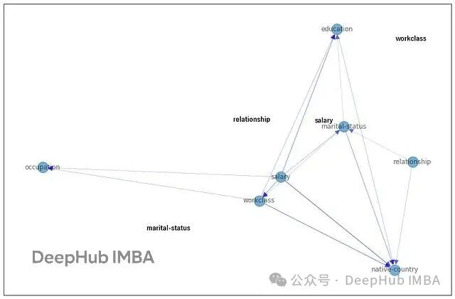
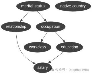
The above figure shows the structure graph learned by <span><span>CausalNex</span></span>. Nodes without labels indicate weak edges that were pruned due to the high threshold. You can also control the sparsity of the network by adjusting the parameter <span><span>w_threshold</span></span> or use <span><span>tabu_edges</span></span> to prohibit certain edges from being generated.
After building the structure, you need to learn the conditional probability distributions for the nodes:
# Step 1: Create BayesianNetwork instance
bn = BayesianNetwork(sm)

# Step 2: Reduce the cardinality of categorical features (optional)
# Step 3: Define the state dictionary for each node
# Step 4: Fit node states
bn = bn.fit_node_states(df)

# Step 5: Fit conditional probability distributions
bn = bn.fit_cpds(df, method="BayesianEstimator", bayes_prior="K2")

# Output CPD for a specific node
result = bn.cpds["education"]
print(result)
<span><span>CausalNex</span></span> has good interpretability and structure learning capabilities, but it has many preprocessing requirements, strict type limitations, and is picky about Python versions (only compatible with 3.6–3.10). If you only want to run standard data, it performs stably, but integrating it into a more complex production environment requires additional work.
4. DoWhy
<span><span>DoWhy</span></span> is a library focused on causal inference validation, with a design philosophy completely different from the previously mentioned Bayesian network tools. It does not attempt to learn causal graphs directly from data but requires users to explicitly define causal assumptions, including:
-
Outcome variable
-
Treatment variable
-
Potential confounding variables
In other words, <span><span>DoWhy</span></span> is more like a validation framework used to systematically question and test your proposed causal assumptions, rather than generating causal structures.
If a DAG (causal graph) is not provided, it will automatically connect all variables to the outcome and treatment variables. However, in practical use, it is best to combine domain knowledge to define the DAG yourself; otherwise, the model will oversimplify.
Using the same Census Income dataset, the treatment variable is defined as “having a doctoral degree”:
# Install
pip install dowhy

# Import libraries
from dowhy import CausalModel
import dowhy.datasets
import datazets as dz
from sklearn.preprocessing import LabelEncoder
import numpy as np
le = LabelEncoder()

# Import data and remove continuous and sensitive features
df = dz.get(data='census_income')

drop_cols = ['age', 'fnlwgt', 'education-num', 'capital-gain', 'capital-loss', 'hours-per-week', 'race', 'sex']
df.drop(labels=drop_cols, axis=1, inplace=True)

# Treatment variable must be binary
df['education'] = df['education']=='Doctorate'

# Convert data to numeric
df_num = df.copy()
for col in df_num.columns:
    df_num[col] = le.fit_transform(df_num[col])

# Specify treatment variable, outcome variable, and potential confounding variables
treatment = "education"
outcome = "salary"

# Step 1: Create causal graph
model = CausalModel(
        data=df_num,
        treatment=treatment,
        outcome=outcome,
        common_causes=list(df.columns[~np.isin(df.columns, [treatment, outcome])]),
        graph_builder='ges',
        alpha=0.05,
        )

# View model
model.view_model()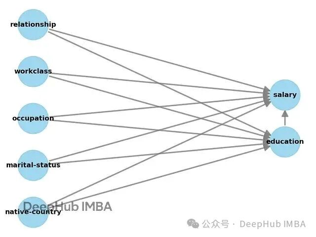
The above figure shows the DAG automatically generated by <span><span>DoWhy</span></span>, where the outcome variable is “salary” and the treatment variable is “education”. It can be seen that the model assumes that education level affects salary, and both may be influenced by confounding factors such as marital status and job type.
The next steps are to identify and estimate causal effects:
# Step 2: Identify causal effect
identified_estimand = model.identify_effect(proceed_when_unidentifiable=True)
print(identified_estimand)
Once the model identifies the estimable causal effect, the average treatment effect (ATE) can be calculated:
 # Step 3: Estimate effect
estimate = model.estimate_effect(identified_estimand, method_name="backdoor.propensity_score_stratification")
print(estimate)
The output average effect value is approximately 0.47, indicating a significant positive causal relationship between a doctoral degree and high income. Finally, a robustness check is performed:
# Step 4: Robustness verification
refute_results = model.refute_estimate(identified_estimand, estimate, method_name="random_common_cause")
DoWhy is very common in academia, with the advantage of a clear framework, transparent assumptions, and complete verification logic; the downside is that it has high input requirements (variables need to be binary, categories need to be numerically encoded), and it cannot automatically learn structures from data.
In other words, it assumes that you already know the potential causal relationships and just want to verify whether this assumption is reasonable.
5. PyAgrum
<span><span>PyAgrum</span></span> is another relatively complete probabilistic graphical model library. It supports the construction of Bayesian networks, Markov networks, and decision graphs, and can perform structure learning, parameter learning, inference, and visualization. Its syntax is more engineering-oriented, making it somewhat more intuitive than <span><span>pgmpy</span></span>, but it requires all variables to be discrete.
If there are missing values or continuous variables in the data, they need to be processed; otherwise, the algorithm will throw an error. The following example demonstrates the complete process from data cleaning to structure learning:
# Install
pip install pyagrum

# Optional: Install visualization dependencies
pip install setgraphviz

import datazets as dz
import pandas as pd
import pyagrum as gum
import pyagrum.lib.notebook as gnb
import pyagrum.lib.explain as explain
import pyagrum.lib.bn_vs_bn as bnvsbn

# Import visualization settings
from setgraphviz import setgraphviz
setgraphviz()

# Import data and remove continuous and sensitive features
df = dz.get(data='census_income')

drop_cols = ['age', 'fnlwgt', 'education-num', 'capital-gain', 'capital-loss', 'hours-per-week', 'race', 'sex']
df.drop(labels=drop_cols, axis=1, inplace=True)

# Clean missing values
df2 = df.dropna().copy()
df2 = df2.fillna("missing").replace("?", "missing")

# Convert all columns to categorical type
for col in df2.columns:
    df2[col] = df2[col].astype("category")

# Create learner
learner = gum.BNLearner(df2)
learner.useScoreBIC()
learner.useGreedyHillClimbing()

# Learn structure
bn = learner.learnBN()

# Learn parameters
bn2 = learner.learnParameters(bn.dag())

# Visualize results
gnb.showBN(bn2)
The above figure shows the Bayesian network structure learned by <span><span>PyAgrum</span></span>. The arrows between nodes indicate potential causal directions.
It provides a series of auxiliary modules to compare different structures (<span><span>bn_vs_bn</span></span>), explain individual nodes (<span><span>explain</span></span>), or generate reports.
<span><span>PyAgrum</span></span> features include: transparent learning process, support for constraint learning (can specify prohibited/mandatory edges), but the cost is that input preparation is relatively cumbersome. There is no automatic missing value handling, continuous features must be discretized, and some functions depend on Graphviz for visualization.
6. CausalImpact
<span><span>CausalImpact</span></span> was originally an open-source project by Google, used to measure intervention effects through Bayesian structural time series models. It differs from the previous libraries in that it does not learn causal graphs but calculates the quantifiable impact of interventions on time series data.
Common scenarios include evaluating the effects of marketing campaigns, price adjustments, or the launch of new features. For example, an e-commerce website wants to know whether an advertising campaign has led to actual sales increases.<span><span>CausalImpact</span></span> first establishes a baseline model using pre-intervention data, then compares the actual observations after the intervention with the predicted values to calculate the “counterfactual difference”.
Below is a concise example, constructing 100 sample points and artificially introducing an intervention effect after the 71st time point:
# Install
pip install causalimpact

# Import libraries
import numpy as np
import pandas as pd
from statsmodels.tsa.arima_process import arma_generate_sample
import matplotlib.pyplot as plt
from causalimpact import CausalImpact

# Generate samples
x1 = arma_generate_sample(ar=[0.999], ma=[0.9], nsample=100) + 100
y = 1.2 * x1 + np.random.randn(100)
y[71:] = y[71:] + 10
data = pd.DataFrame(np.array([y, x1]).T, columns=["y","x1"])

# Initialize model
impact = CausalImpact(data, pre_period=[0,69], post_period=[71,99])

# Perform inference
impact.run()

# Plotting and results
impact.plot()
impact.summary()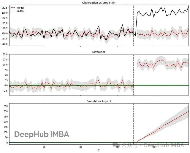
The upper part of the figure shows the comparison between actual values and model predictions; the middle part is the difference between the two (instantaneous effect); the lower part is the cumulative effect.
The results show that the intervention led to a significant increase, with a probability of 100% and a p-value of 0. This method assumes that the relationship between covariates and response variables remains stable before and after the intervention, and that the covariates themselves are not affected by the intervention. If these assumptions are met, <span><span>CausalImpact</span></span> is very reliable for quantitatively assessing intervention effects.
Summary
The six libraries have very different approaches. Overall, they can be divided into two categories:
Structure Learning Type:<span><span>Bnlearn</span></span>, <span><span>Pgmpy</span></span>, <span><span>CausalNex</span></span>, and <span><span>PyAgrum</span></span> are used to discover potential causal relationships between variables, suitable for exploratory analysis and structural modeling.
Causal Effect Type:<span><span>DoWhy</span></span> and <span><span>CausalImpact</span></span> focus on quantifying intervention effects given a structure or time series, suitable for policy analysis or experimental validation.
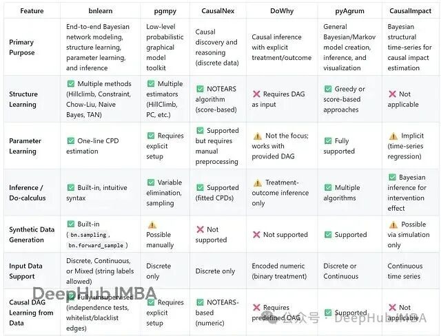
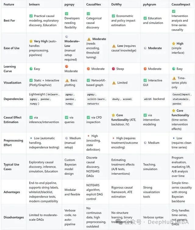
From an engineering perspective:<span><span>Bnlearn</span></span> has the highest ease of use, with a friendly interface and strong compatibility, making it a good tool for beginners and quick validation;<span><span>Pgmpy</span></span> has the strongest flexibility, suitable for in-depth research and custom algorithms;<span><span>CausalNex</span></span> has a good interpretable graphical interface but relies on specific Python versions;<span><span>DoWhy</span></span> is a commonly used tool in academic research, emphasizing theoretical rigor;<span><span>PyAgrum</span></span> is stable and transparent, but data preparation is relatively heavy;<span><span>CausalImpact</span></span> focuses on causal evaluation of time series.
The six causal libraries cover the complete path from structure learning to causal effect estimation.
<span><span>Bnlearn</span></span>, <span><span>Pgmpy</span></span>, <span><span>CausalNex</span></span> and <span><span>PyAgrum</span></span> are responsible for building networks and identifying driver factors;
<span><span>DoWhy</span></span> and <span><span>CausalImpact</span></span> are more like “quantification tools” used to assess the actual impact of treatments or interventions.
Author: Erdogan T
Editor: Wenjing
About Us
Data Hub THU, as a data science public account, is backed by the Tsinghua University Big Data Research Center, sharing cutting-edge data science and big data technology innovation research dynamics, continuously disseminating data science knowledge, striving to build a platform for gathering data talent, and creating the strongest group in China’s big data.

Weibo: @Data Hub THU
WeChat Video Account: Data Hub THU
Today’s Headlines: Data Hub THU