This article reviews concepts such as the attention mechanism.

Self-Attention

The concept of “attention” originated from efforts to improve Recurrent Neural Networks (RNNs) to handle longer sequences or sentences. For example, consider translating a sentence from one language to another. Word-for-word translation is often impractical as it ignores the complex grammatical structures and idiomatic expressions unique to each language, leading to inaccurate or nonsensical translations.

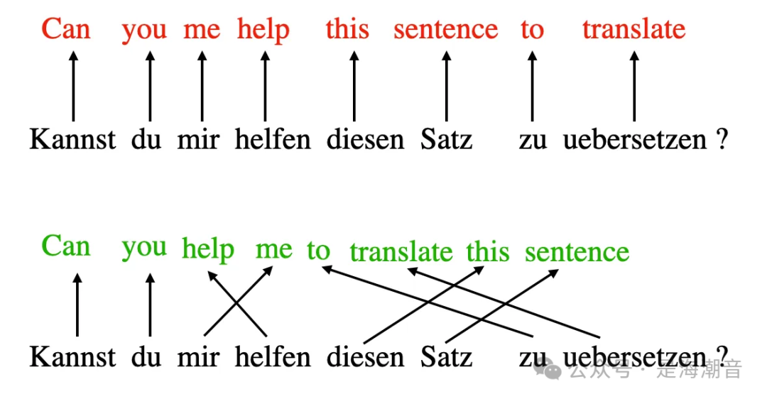
To address this issue, the attention mechanism was introduced to capture all elements of the sequence at each time step. The key is to be selective and determine which words are most important in a given context. In 2017, the Transformer architecture introduced an independent self-attention mechanism, completely eliminating the need for RNNs.

We can think of self-attention as a mechanism that enhances the information content of the input embedding by incorporating contextual information from the input. In other words, the self-attention mechanism allows the model to weigh the importance of different elements in the input sequence and dynamically adjust their influence on the output. This is particularly important in language processing tasks, as the meaning of a word can change depending on its context within a sentence or document.

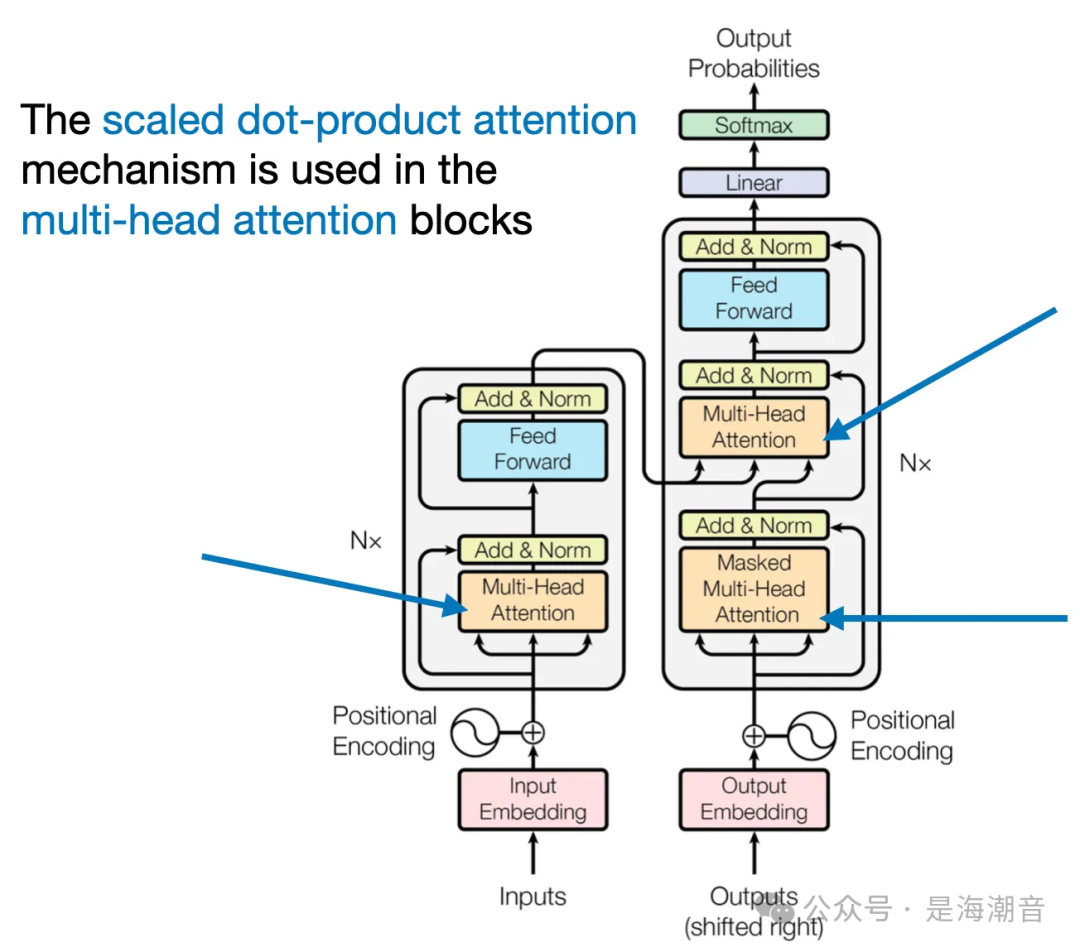
Note that self-attention mechanisms have many variants. A particular focus of research is on improving the efficiency of self-attention. However, most papers still adopt the original scaled-dot product attention mechanism proposed in the paper “Attention Is All You Need”.

If you are interested in other types of attention mechanisms, you can refer to:

• 2020 Efficient Transformers: A Survey
• 2023 A Survey on Efficient Training of Transformers review
• FlashAttention and FlashAttention-v2 papers.

Embedding an Input Sentence

Embedding sizes typically range from hundreds to thousands. For example, the embedding dimension used by Llama 2 is 4096. Here, we demonstrate with 3.

torch.manual_seed(42)
embed = torch.nn.Embedding(vocab_size, 3)
embedded_sentence = embed(sentence_int).detach()

Defining the Weight Matrices

Self-attention uses three weight matrices, referred to as W_q, W_k, and W_v, which are adjusted as model parameters during training. These matrices are used to project the input into the sequence’s query, key, and value.

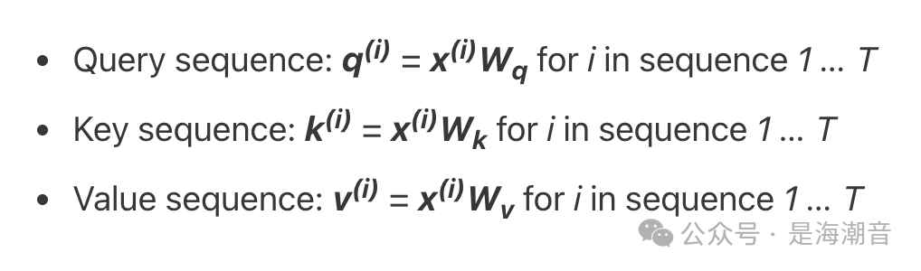
q(i) and k(i) are both vectors of dimension d_k, where d represents the size of each word vector.

Since we need to compute the dot product between Q and K, these two vectors must contain the same number of elements (d_q = d_k). In many LLMs, we use the same size for V, making d_q = d_k = d_v. However, the number of elements in v(i) (which determines the size of the resulting context vector) can be arbitrary.

torch.manual_seed(123)

d = embedded_sentence.shape[1]
# set dq = dk = 2 and use dv = 4,
d_q, d_k, d_v = 2, 2, 4

W_query = torch.nn.Parameter(torch.rand(d, d_q))
W_key = torch.nn.Parameter(torch.rand(d, d_k))
W_value = torch.nn.Parameter(torch.rand(d, d_v))

Computing the Unnormalized Attention Weights

keys = embedded_sentence @ W_key
values = embedded_sentence @ W_value

omega_2 = query_2 @ keys.T

We compute ωi,j as the dot product between the query sequence and the key sequence, i.e., ω_i,j = q⁽ⁱ⁾ k^(j).

Computing the Attention Weights

The next step is to normalize the unnormalized attention weights ω by applying the softmax function to obtain the normalized attention weights α. Before normalizing ω through the softmax function, we scale it by 1/√d_k:

Dividing by d_k ensures that the Euclidean length of the weight vectors will be approximately of the same magnitude. This helps prevent the attention weights from becoming too small or too large, which could lead to numerical instability or affect the model’s convergence during training.

import torch.nn.functional as F

attention_weights_2 = F.softmax(omega_2 / d_k**0.5, dim=0)
print(attention_weights_2)

Why Scale by √dₖ?

Scaling by √dₖ is to stabilize the values of Q·Kᵀ, preventing softmax saturation, thus making training more stable and faster.

1. To avoid excessively large dot products that lead to vanishing gradients in softmax.

Assuming each dimension of Q and K follows a distribution with mean 0 and variance 1. As the dimension dₖ increases:the expected variance of Q·Kᵀ increases with dₖ, leading to larger values (which can be both positive and negative).

Softmax is very sensitive to large values: if scaling is not applied, the dot product results can be very large, causing softmax saturation, which in turn leads to gradients approaching 0, ultimately resulting in unstable training and slower convergence.

Thus, by dividing by √dₖ:

it brings the variance of Q·Kᵀ back to a suitable scale, improving the stability of softmax.

1. Mathematically, scaling makes it more “smooth”, avoiding extreme attention.

If not scaled: the softmax output would be very “sharp” (one token scores particularly high), causing attention weights to be very extreme, making the model hard to optimize.

Scaling is akin to “lowering the temperature”, making softmax smoother and learning more stable.

1. Consistent with weight initialization logic.

Common initializations in neural networks, such as Xavier / Kaiming initialization, include similar divisions by √d:

• Maintaining stable variance in forward and backward passes.
• Preventing gradient explosion/vanishing.

The scaling in attention follows the same reasoning.

Why is the scaling factor √dₖ and not dₖ?

1. The key reason: variance grows linearly with dimension dₖ.

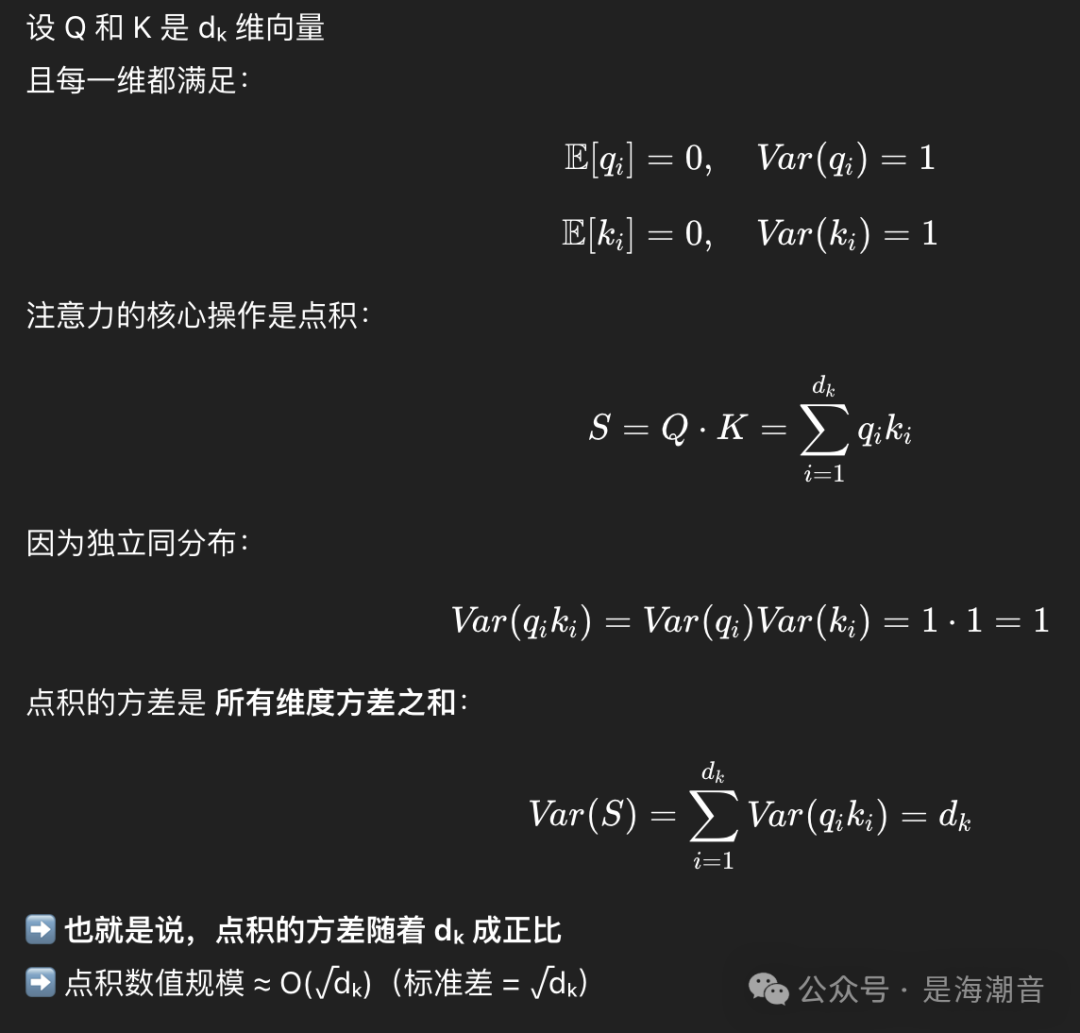
1. The scale of softmax inputs is determined by the standard deviation (not variance).

The saturation of softmax depends on the absolute size of the input values, which is proportional to the standard deviation σ = √Var.

The standard deviation of the dot product S:

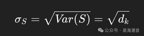
If not scaled, the typical magnitude of S would be about √dₖ. Therefore, the appropriate scaling method is to divide by √dₖ, not dₖ.

What Happens if Divided by dₖ?

• (1) Softmax becomes too smooth — attention degrades.

Softmax inputs become very small, leading to softmax approaching a uniform distribution, causing attention weights to trend towards average, making it ineffective to “focus”.

• (2) Gradients become too small → model training becomes difficult. Softmax behaves almost linearly for small inputs, resulting in very small gradients, and the attention module becomes nearly ineffective, causing a sharp decline in Transformer performance.

Original Explanation

“We scale the dot products by 1/√dₖ to counteract the effect of large dot-product magnitudes which can push the softmax function into regions where it has extremely small gradients.”

We use 1/√dₖ to scale the dot product to counteract the effect of large values from high-dimensional vector dot products, as excessively large values can push softmax into regions with very small gradients.

Computing with Value Vector

The final step is to compute the context vector z(2), which is the attention-weighted version of our original query input x(2), incorporating all other input elements as its context through the attention weights:

context_vector_2 = attention_weights_2 @ values

Self-Attention in Code

import torch.nn as nn
class SelfAttention(nn.Module):
    def __init__(self, d_in, d_out_kq, d_out_v):
        super().__init__()
        self.d_out_kq = d_out_kq
        self.W_query = nn.Parameter(torch.rand(d_in, d_out_kq))
        self.W_key   = nn.Parameter(torch.rand(d_in, d_out_kq))
        self.W_value = nn.Parameter(torch.rand(d_in, d_out_v))
    # @ is the matrix multiplication operator introduced in Python 3.5. It is equivalent to:
    # torch.matmul(x, W_key) (in PyTorch)
    # x.dot(W_key) (in some cases in NumPy)
    # Mathematical matrix multiplication 𝑋×𝑊
    
    def forward(self, x):
        keys = x @ self.W_key
        queries = x @ self.W_query
        values = x @ self.W_value
        
        attn_scores = queries @ keys.T  # unnormalized attention weights    
        attn_weights = torch.softmax(
            attn_scores / self.d_out_kq**0.5, dim=-1
        )
        
        context_vec = attn_weights @ values
        return context_vec

Using this class in practice:

torch.manual_seed(123)
# reduce d_out_v from 4 to 1, because we have 4 heads
d_in, d_out_kq, d_out_v = 3, 2, 4
sa = SelfAttention(d_in, d_out_kq, d_out_v)
print(sa(embedded_sentence))

Multi-Head Attention

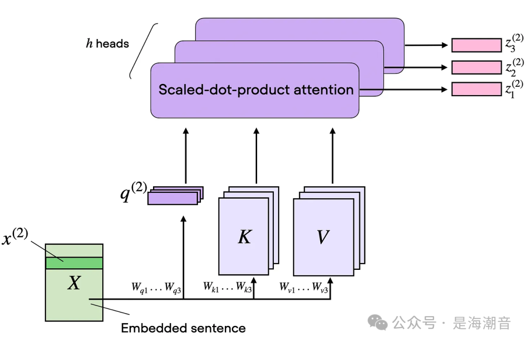
In scaled dot-product attention, the input sequence is transformed through three matrices representing queries, keys, and values. In the context of multi-head attention, these three matrices can be viewed as a single attention head.

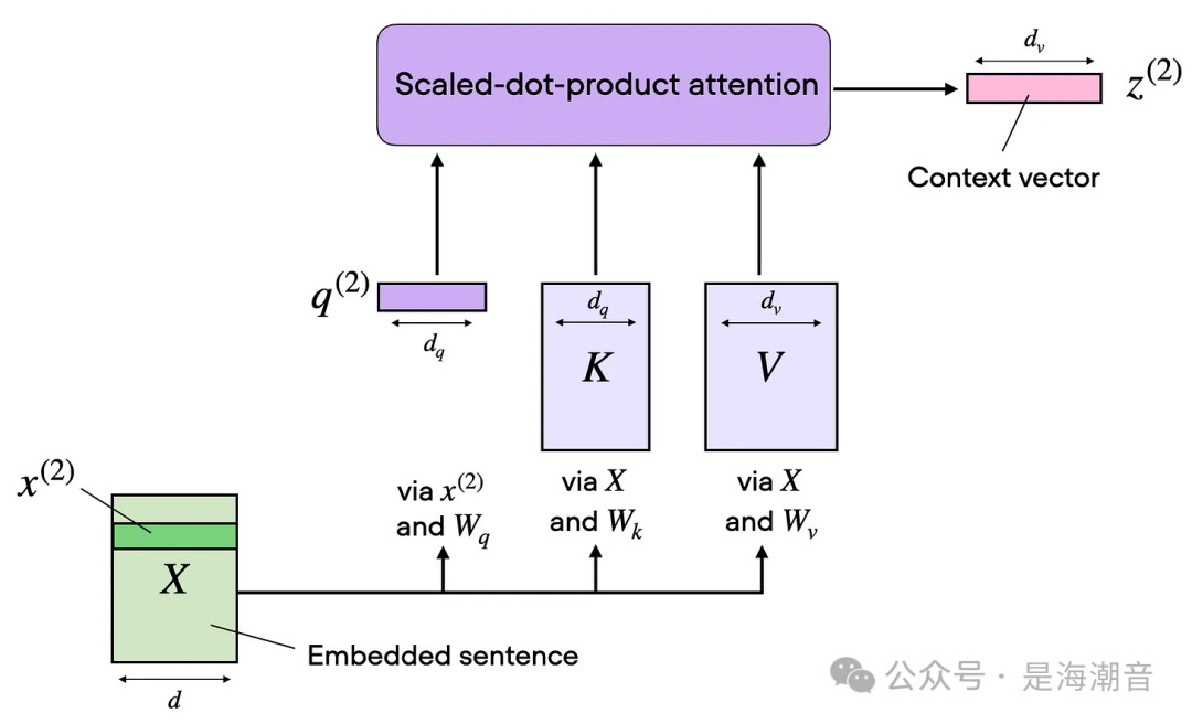
Multi-head attention consists of multiple such heads, each composed of query, key, and value matrices. This concept is similar to the use of multiple kernels in convolutional neural networks, generating feature maps with multiple output channels.

class MultiHeadAttentionWrapper(nn.Module):
    def __init__(self, d_in, d_out_kq, d_out_v, num_heads):
        super().__init__()
        self.heads = nn.ModuleList(
            [SelfAttention(d_in, d_out_kq, d_out_v) 
             for _ in range(num_heads)]
        )
    def forward(self, x):
        return torch.cat([head(x) for head in self.heads], dim=-1)

We initialize the SelfAttention class num_heads times with these input parameters. We use PyTorch’s nn.ModuleList to store these multiple SelfAttention instances.

Then, the forward pass involves applying each SelfAttention head (stored in self.heads) independently to the input x. The results from each head are concatenated along the last dimension (dim=-1).

torch.manual_seed(123)
block_size = embedded_sentence.shape[1]
mha = MultiHeadAttentionWrapper(
    d_in, d_out_kq, d_out_v, num_heads=4
)
context_vecs = mha(embedded_sentence)
print(context_vecs)
print("context_vecs.shape:", context_vecs.shape)

Note that the result of multi-head attention is a tensor of shape 6×4: we have 6 input tokens and 4 self-attention heads, each returning a 1-dimensional output. Previously, we also generated a tensor of shape 6×4 in the self-attention section. This is because we set the output dimension to 4 instead of 1. In practice, if we could adjust the output embedding size within the SelfAttention class itself, why do we need multiple attention heads?

The difference between increasing the output dimension of a single self-attention head and using multiple attention heads lies in how the model processes data and learns from it. While both approaches can enhance the model’s ability to represent different features or aspects of the data, they fundamentally differ in their implementation.

For instance, each attention head in the multi-head attention mechanism has the potential to learn to focus on different parts of the input sequence, capturing various aspects or relationships within the data. Allowing different heads to focus on different semantic patterns: head 1 may focus on syntax; head 2 on distance; head 3 on entities. This diversity in representation is key to the success of the multi-head attention mechanism.

Multi-head attention can also be more efficient, especially in terms of parallel computation. Each head can be processed independently, making it well-suited for modern hardware accelerators like GPUs or TPUs that excel at parallel processing. In short, using multiple attention heads is not only to increase the model’s capacity but also to enhance its ability to learn various features and relationships within the data. For example, the 7B Llama 2 model uses 32 attention heads.

Causal Self-Attention

The causal self-attention mechanism is specifically designed for large language models of the GPT class (decoder-style), which are used for text generation. This causal self-attention mechanism is often referred to as “masked self-attention”. In the original Transformer architecture, it corresponds to the “masked multi-head attention” module.

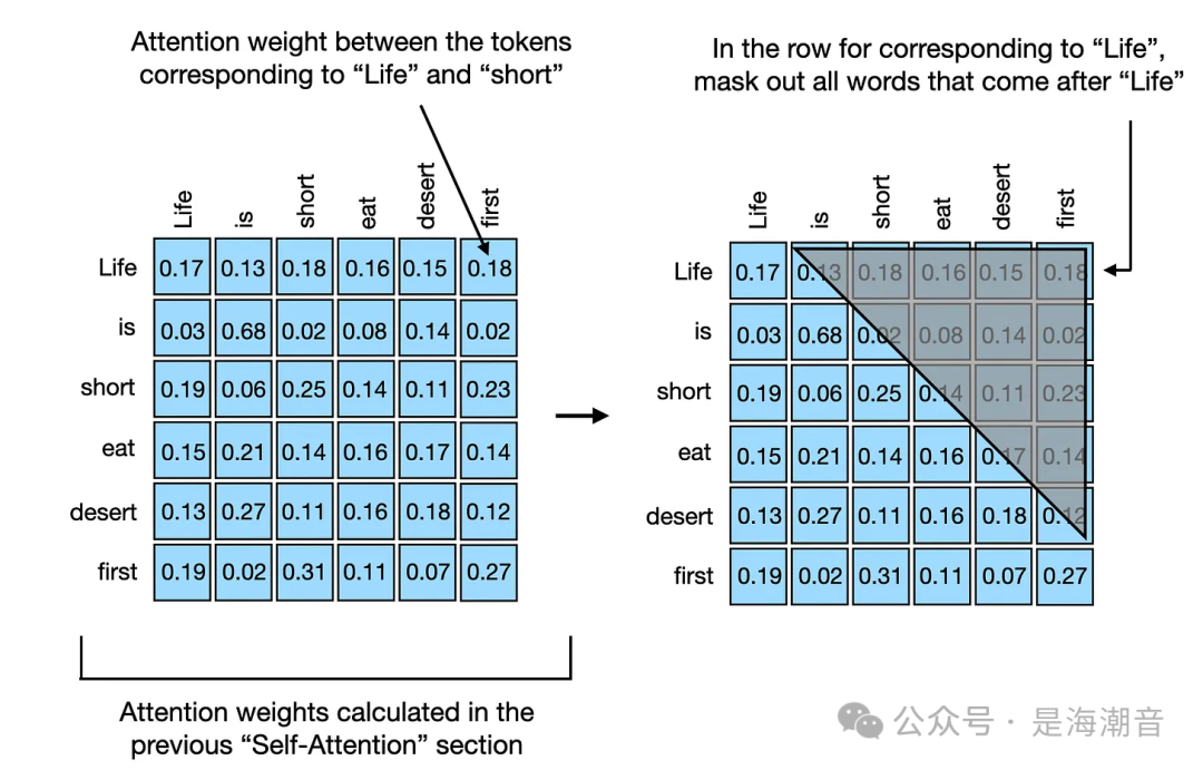
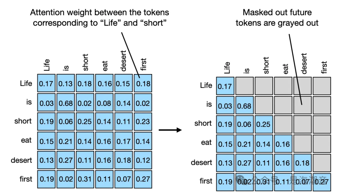
The causal self-attention mechanism ensures that the output at a certain position in the sequence depends only on the known outputs from previous positions, without relying on outputs from future positions. In simple terms, it guarantees that the prediction of each next word should only depend on the preceding words. In large language models like GPT, to achieve this, we mask the future tokens in the input text for each processed token.

The following diagram illustrates the process of hiding future input tokens in the input by applying a causal mask to the attention weights.

The simplest way to implement the above setup is to apply a mask to the attention weight matrix above the diagonal, as shown in the following diagram. This way, when creating the context vector, the “future” words will not be included, and the context vector is obtained by summing the input weighted by attention.

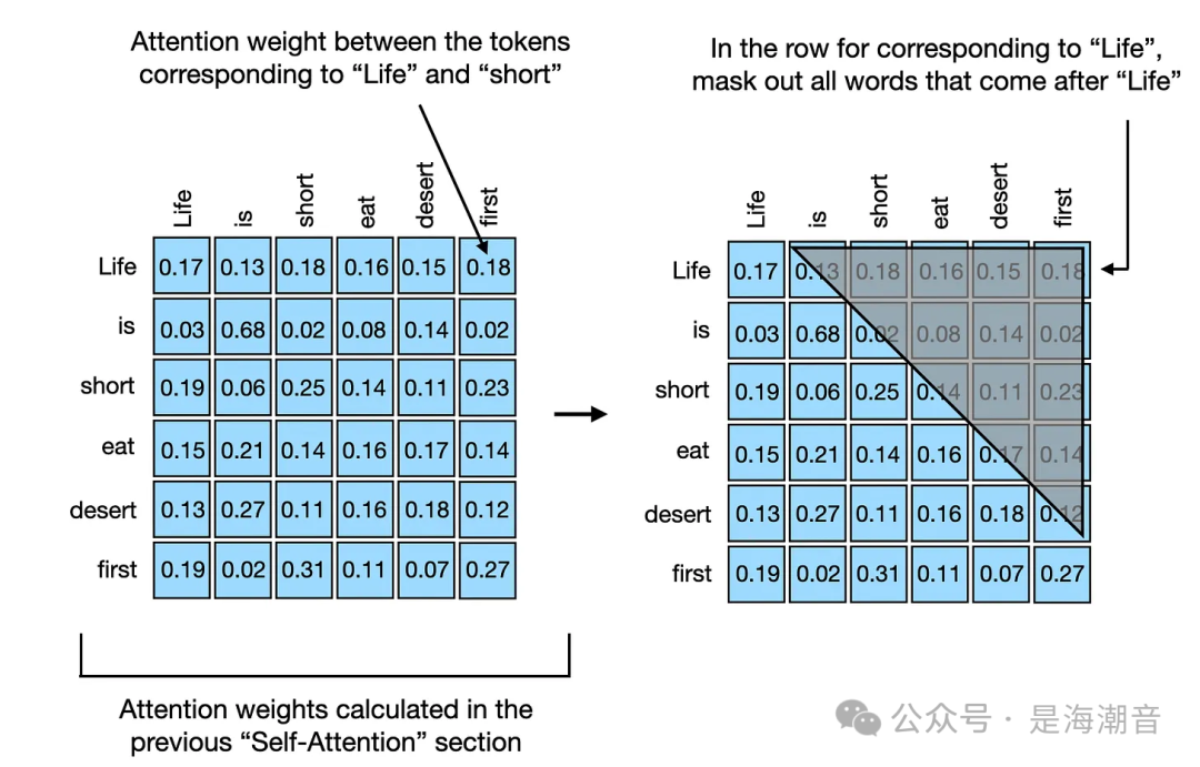
In code, we can achieve this using PyTorch’s tril function to create a mask consisting of 1s and 0s:

block_size = attn_scores.shape[0]
mask_simple = torch.tril(torch.ones(block_size, block_size))
print(mask_simple)
  
# Output
tensor([[1., 0., 0., 0., 0., 0.],
        [1., 1., 0., 0., 0., 0.],
        [1., 1., 1., 0., 0., 0.],
        [1., 1., 1., 1., 0., 0.],
        [1., 1., 1., 1., 1., 0.],
        [1., 1., 1., 1., 1., 1.]])

Next, we multiply the attention weights by this mask to zero out all attention weights above the diagonal:

masked_simple = attn_weights*mask_simple
# Output
tensor([[0.1772, 0.0000, 0.0000, 0.0000, 0.0000, 0.0000],
        [0.0386, 0.6870, 0.0000, 0.0000, 0.0000, 0.0000],
        [0.1965, 0.0618, 0.2506, 0.0000, 0.0000, 0.0000],
        [0.1505, 0.2187, 0.1401, 0.1651, 0.0000, 0.0000],
        [0.1347, 0.2758, 0.1162, 0.1621, 0.1881, 0.0000],
        [0.1973, 0.0247, 0.3102, 0.1132, 0.0751, 0.2794]],
       grad_fn=<MulBackward0>)

While the above is one way to mask future tokens, note that the attention weights for each row no longer sum to 1. To mitigate this issue, we can normalize the rows so that their sums are again 1, which is a standard practice for attention weights:

row_sums = masked_simple.sum(dim=1, keepdim=True)
masked_simple_norm = masked_simple / row_sums
print(masked_simple_norm)

Normalizing attention weights in neural networks (like Transformer models) has two main advantages over unnormalized weights. First, normalized attention weights that sum to 1 resemble a probability distribution, making it easier to interpret the model’s attention on different parts of the input from a proportional perspective. Second, constraining attention weights to sum to 1 helps control the scale of weights and gradients, improving training dynamics.

More Efficient Masking Without Renormalization

A more efficient method is to obtain the attention scores and replace the values above the diagonal with negative infinity before inputting these values into the softmax function to compute the attention weights.

mask = torch.triu(torch.ones(block_size, block_size), diagonal=1)
masked = attn_scores.masked_fill(mask.bool(), -torch.inf)
print(masked)

The above code first creates a mask where the lower part of the diagonal is 0 and the upper part is 1. Here, torch.triu (upper triangle) retains the elements of the matrix diagonal and above, setting the lower elements to 0, thus preserving the upper triangular part. In contrast, torch.tril (lower triangle) retains the elements of the main diagonal and below.

Then, we simply apply the softmax function as usual to obtain normalized and masked attention weights:

attn_weights = torch.softmax(masked / d_out_kq**0.5, dim=1)

Why is this? The final step of applying the softmax function converts the input values into a probability distribution. When there are -inf values in the input, softmax effectively treats them as zero probability. This is because e^(-inf) approaches 0, so these positions contribute nothing to the output probabilities.