01Introduction
This academic sharing is based on the research work published by researchers from Xi’an University of Electronic Science and Technology in IEEE TRANSACTIONS ON VEHICULAR TECHNOLOGY in 2019.
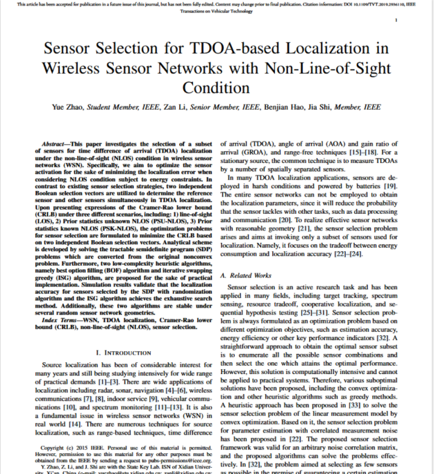
Paper Title: Sensor Selection for TDOA-based Localization in Wireless Sensor Networks with Non-Line-of-Sight Condition
Authors:Yue Zhao, Student Member, IEEE, Zan Li, Senior Member, IEEE, Benjian Hao, Jia Shi
Source:《IEEE TRANSACTIONS ON VEHICULAR TECHNOLOGY》,IF:6.1,中科院JCR分区2区TOP期刊,DOI:10.1109/TVT.2019.2936110
Value Rating:
Innovation:★★★★★:
The paper first proposes a dual independent Boolean selection vector (distinguishing reference sensors from ordinary sensors), breaking through the confusion of traditional single vector selection; constructs a CRLB (Cramér-Rao Lower Bound) optimization framework under three scenarios: LOS/PSU-NLOS/PSK-NLOS, innovatively transforming the non-convex sensor selection problem into a semidefinite programming (SDP) problem, while proposing a low-complexity heuristic algorithm (BOF/ISG), significantly different from traditional models that only cover LOS scenarios or single-type sensor selection.
Engineering Value:★★★★☆:
The paper verifies the effectiveness of the SDP algorithm (theoretical optimal) and the ISG algorithm (near-optimal) through simulations. The complexity of the ISG algorithm is only O(S²) (S is the total number of sensors), making it suitable for resource-constrained WSNs (such as low-power IoT nodes); the sensor selection strategy under energy constraints can balance positioning accuracy and node lifespan, requiring only a rough source location estimate in practical deployment, demonstrating strong engineering feasibility.
Theoretical Depth:★★★★☆:
The paper derives analytical expressions for CRLB/G-CRLB (Generalized CRLB) under three scenarios, clarifying the mechanism of NLOS errors affecting positioning accuracy; it transforms the non-convex optimization problem into a convex SDP problem using the Schur complement lemma, proving the near-optimality of the relaxed solution; analyzes the convergence and complexity of the BOF/ISG algorithms, forming a complete theoretical chain of “modeling – optimization – verification”.
Further Reading:
1. Extension: AOA Sensor Placement for Anchor-Assisted Target Localization in GNSS-Denied Environment: Formulation, Bounds and Optimization focuses on sensor deployment based on AOA in GNSS-denied environments, solving the unknown sensor location problem with anchor assistance, deriving the joint CRLB lower bound for sensors and targets, and proposing the SPSA-Adam optimization algorithm. This complements the current work (TDOA+NLOS) by covering mainstream positioning technology sensor selection needs in WSN.
2. Extension: Z. Dai et al., “Nearly Optimal Sensor Selection for TDOA-Based Source Localization in Wireless Sensor Networks,” IEEE Transactions on Vehicular Technology, vol. 69, no. 10, pp. 12031-12042, 2020. proposes two near-optimal algorithms, SDR-TDOA and SDR-TOA, which achieve sensor selection using a single Boolean vector (without distinguishing between reference and ordinary sensors), simplifying the optimization model by proving the equivalence of “TDOA-CRLB and TOA-CRLB with unknown transmission time.” This contrasts with the current paper’s “dual Boolean vector” design, providing a more straightforward convex relaxation approach, reducing complexity, and making it suitable for large-scale WSN scenarios, and this paper later addresses dynamic situations.
3. Main Content: Dual Boolean Selection Vector Design: Define vectors q and p, through 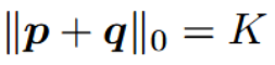 and
and 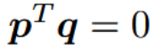 constraints, solving the defect of traditional single vector that cannot distinguish reference nodes.
4. Scenario-specific CRLB Modeling:
1) LOS Scenario: Only considering TDOA measurement noise, CRLB is represented by the inverse of the Fisher Information Matrix (FIM); 2) PSU-NLOS Scenario (NLOS prior unknown): Proves that positioning accuracy only relies on LOS sensors, with NLOS sensors contributing nothing; 3) PSK-NLOS Scenario (NLOS prior known): Introduces a prior information matrix , constructing G-CRLB to utilize NLOS sensors to improve accuracy.
5. Algorithm System Construction: 1) Proposes the SDP benchmark algorithm: transforms the non-convex problem into a solvable SDP through convex relaxation, combined with randomization methods to obtain Boolean solutions; 2) Proposes low-complexity heuristic algorithms: BOF (stepwise addition of sensors) and ISG (iterative exchange of sensors), meeting real-time deployment needs;
6. Experimental Verification: Validates the positioning accuracy of the ISG algorithm under different numbers of sensors, noise intensities, and NLOS ratios, showing that the ISG algorithm’s accuracy is close to that of the exhaustive method (optimal but with extremely high complexity), and significantly better than the “nearest sensor method” and “random selection method.”
7. Research Gene Analysis: The TDOA positioning principle infers the source location from the time difference of signals received by multiple sensors, forming the basis of the system modeling in this paper, as shown in formula (1).

CRLB/G-CRLB lower bound theory: provides theoretical limits for the minimum variance of unbiased estimates, and in NLOS scenarios, it needs to be combined with error priors to extend to G-CRLB, which is the core indicator for accuracy assessment in this paper; convex optimization (SDP): relaxes non-convex Boolean constraints through semidefinite programming, a classic tool for solving combinatorial optimization problems, providing methodological support for the SDP benchmark algorithm in this paper.
The paper first separates reference and ordinary sensor selection, ensuring the uniqueness of reference nodes through orthogonal constraints, optimizing positioning geometry; models for LOS/PSU-NLOS/PSK-NLOS scenarios are established, clarifying the sensor selection logic under different scenarios; and the SDP provides a theoretically optimal benchmark, while BOF/ISG balances accuracy and complexity, adapting to different engineering needs.
02Literature Background
With the widespread application of WSN in fields such as radar, navigation, and vehicular communication, TDOA positioning has become a mainstream technology due to its lack of need for synchronized clocks. However, it faces two core challenges in practical scenarios: NLOS propagation interference: In indoor/rural scenarios, obstacles cause non-line-of-sight propagation of signals, leading to path errors, with positioning errors exceeding 30% under traditional LOS assumptions; reference sensor blind spots: TDOA positioning relies on reference sensors, and fixed reference nodes may lead to pathological geometry (e.g., when the reference node is far from the source, TDOA measurement noise is amplified), and traditional single vector selection cannot solve this problem.
Therefore, the core problem addressed by this research is: how to minimize positioning errors (using CRLB as an indicator) through sensor selection in WSN-TDOA positioning under NLOS conditions, adapting to different NLOS scenarios (prior known/unknown), while solving the geometric adaptation and high complexity issues of traditional algorithms:
Problem Definition:
(1) System Model
WSN Structure: S sensors , source location
 ; NLOS sensor set
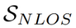 , LOS sensor set
 ;
;
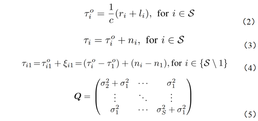
TOA/TDOA Measurement Model: TOA true value, TOA measurement value, TDOA measurement value, noise covariance matrix Q as follows
(2) Three Scenario CRLB Modeling
LOS Scenario (CRLB_L): Only considering measurement noise, CRLB is the inverse of FIM:
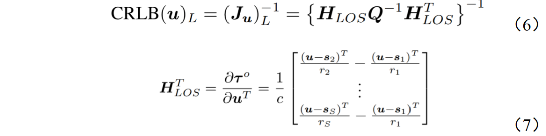
Reflects the impact of geometry and noise on accuracy.
PSU-NLOS Scenario: Unknown parameters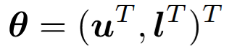 (including source location and NLOS error), CRLB is
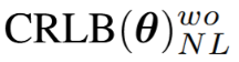 left upper 3×3 block (only source location part), and only relies on LOS sensors, its formula is

PSK-NLOS Scenario (G-CRLB): combines NLOS prior information for NLOS error standard deviation), FIM is extended to , CRLB is the source location part of its inverse matrix, utilizing NLOS priors to reduce errors.
03Research Methodology
1. System Model Design
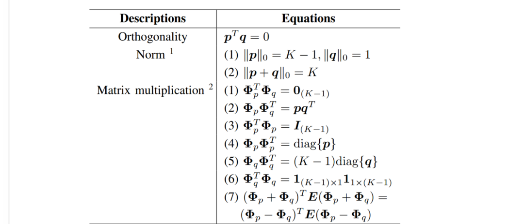
Dual Boolean Vector Framework: Separates selection through q (reference sensors) and p (ordinary sensors), defining matrices Φp (extracting ordinary sensors) and Φq (expanding reference sensors), ensuring that the FIM and noise matrix of selected sensors can be accurately calculated; the following table shows the vector attributes.
2. Algorithm Design
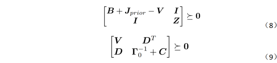
(1) SDP Benchmark Algorithm (theoretical optimal) addresses the non-convexity of constraints P1-P3 by transforming it into SDP for computation. Introduces auxiliary matrices: defines Z (replacing the inverse matrix of CRLB) and V (simplifying inverse operations), transforming non-convex constraints into linear matrix inequalities (LMI) through the Schur complement lemma:
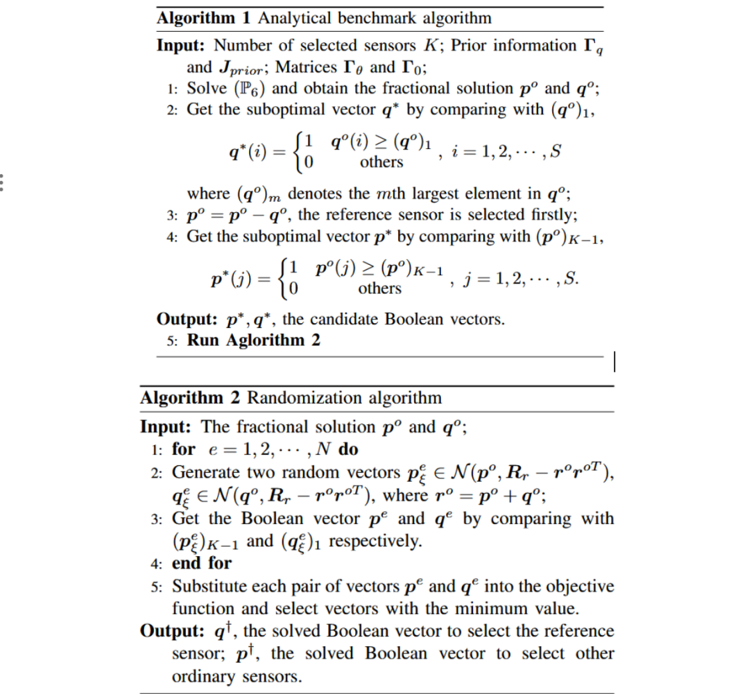
 Relaxation and randomization: relaxes the Boolean constraints p,q∈{0,1}^S to p,q∈[0,1]^S, solving it and obtaining Boolean solutions through randomization methods (generating N=50 sets of random vectors) to ensure near-optimality. The SDP benchmark algorithm is as follows:
(2) Low-complexity Heuristic Algorithms
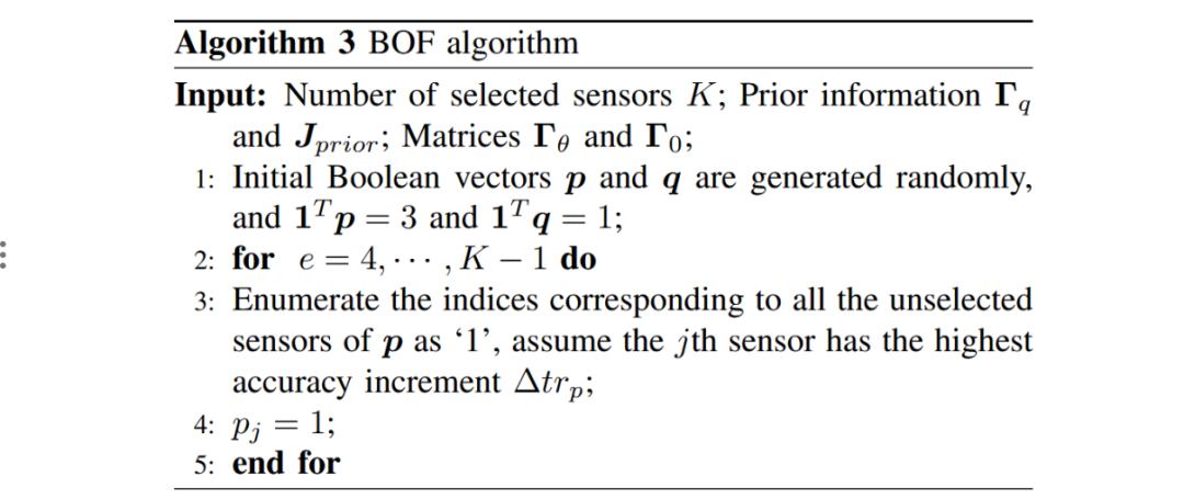
To meet real-time deployment needs, two algorithms BOF and ISG are proposed: BOF algorithm (stepwise filling): the initial subset consists of 3 ordinary sensors and 1 reference sensor, each time enumerating unselected sensors, selecting the sensor that maximally decreases CRLB to add, until the total is K, with complexity O(S²); the BOF algorithm is as follows:
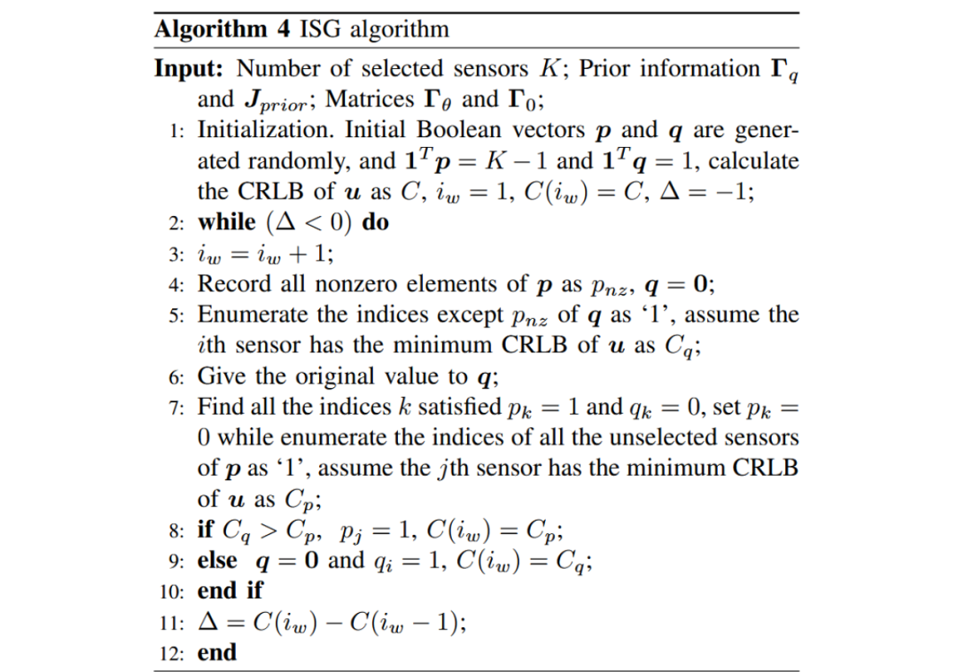
(3) ISG Algorithm (Iterative Exchange): The initial subset consists of K random sensors, each time exchanging “selected – unselected” sensors, comparing the CRLB of “ordinary sensor exchange” and “reference sensor exchange,” selecting the optimal exchange until CRLB no longer decreases, converging quickly, with accuracy close to that of the exhaustive method. The ISG algorithm is as follows:
03Experimental Verification
1) Experimental Setup:
WSN Configuration: S=30/100 sensors, position coordinates follow N(0,3000000); source location 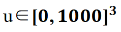 (static); number of NLOS sensors M=5/10/15; noise model: TOA noise
  ,
, corresponding ROA noise intensity −5∼10dB; exhaustive method (optimal), SDP + randomization, BOF, ISG, nearest sensor method, random selection method; evaluation metrics: CRLB (m², the smaller the better), coverage rate (Cv, proportion of covered users), success rate (SR, proportion of experimental times where CRLB≤threshold); reliability verification: 200 Monte Carlo experiments averaged, excluding random geometry and noise interference.
2) Key Experimental Results
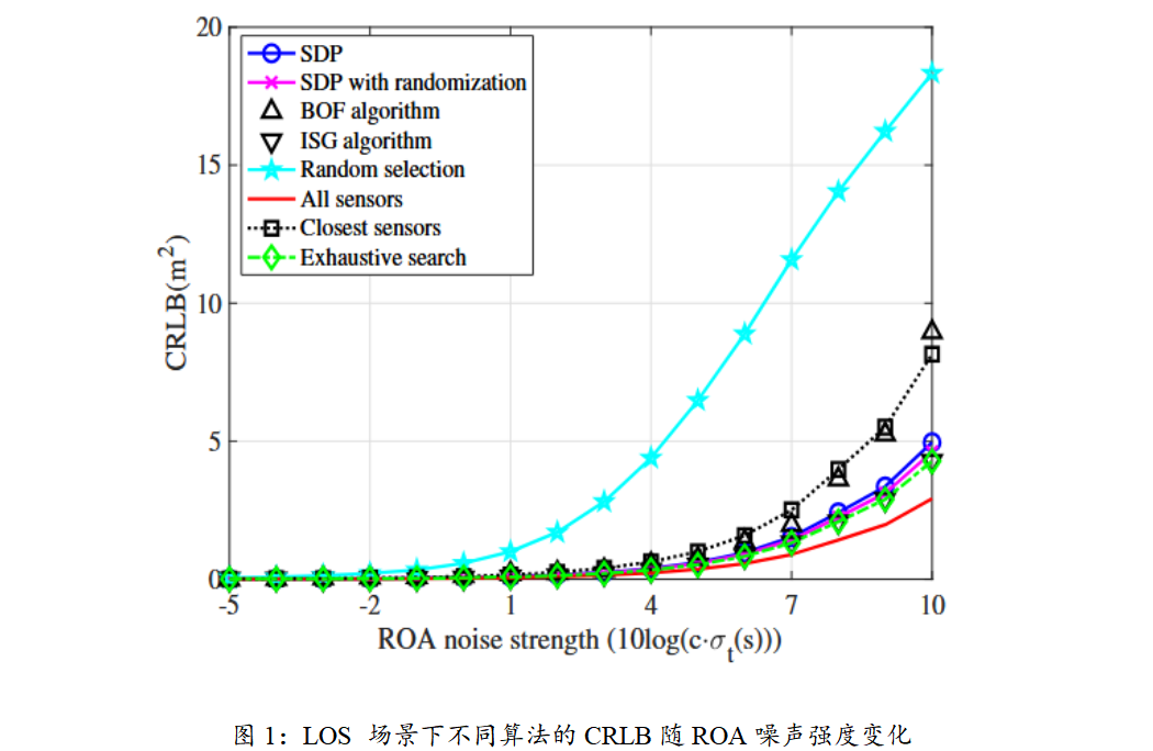
LOS Scenario (S=30, K=8): Relationship between CRLB and noise intensity: As shown in Figure 1, CRLB monotonically increases with the increase of ROA noise intensity, but the ISG algorithm remains close to the exhaustive method (error < 2%), while the nearest sensor method has an error exceeding 50%. When ROA=-5dB, ISG’s CRLB=8.3m², only 1.2% higher than the exhaustive method; when ROA=10dB, ISG’s CRLB=18.8m², still 33.6% lower than the nearest sensor method. The results are shown in Figure 1.
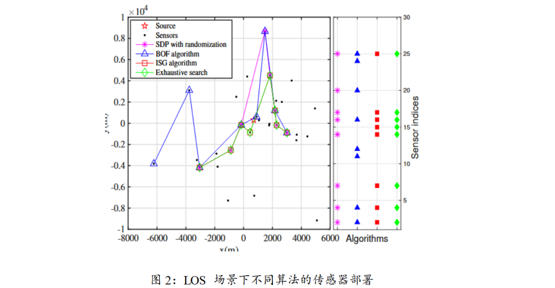
ISG algorithm selected sensors are identical to those of the exhaustive method, uniformly distributed around the source, with reference sensors approximately 1500m from the source, avoiding pathological geometry; while the BOF algorithm, due to the influence of the initial random subset, selects sensors concentrated on the right side, and the nearest sensor method only selects local sensors near the source, leading to decreased positioning accuracy. As shown in the following figure.
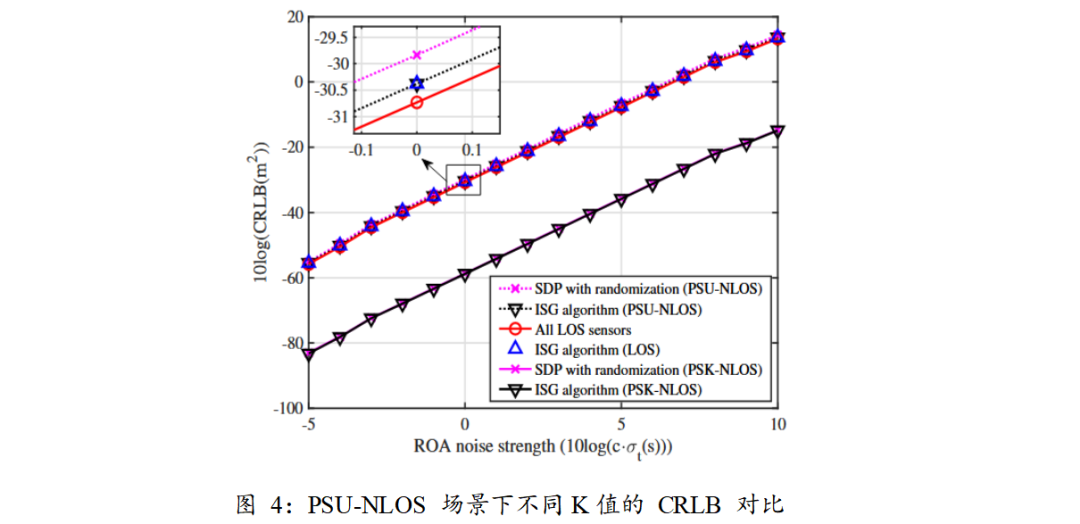
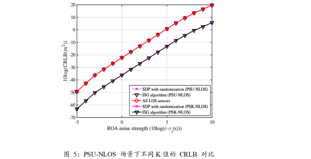
PSK-NLOS Scenario (S=30, K=8, M=5) CRLB Comparison: As shown in Figure 3, in the PSK-NLOS scenario, the ISG algorithm still maintains optimal performance — when ROA=10dB, ISG’s CRLB=19.5m², 18% lower than the PSU-NLOS scenario (only selecting LOS sensors, CRLB=23.8m²), proving that NLOS prior information can effectively improve accuracy; while the random selection method, due to including 2-3 NLOS sensors, has a CRLB of 32.1m², with an error exceeding 60%.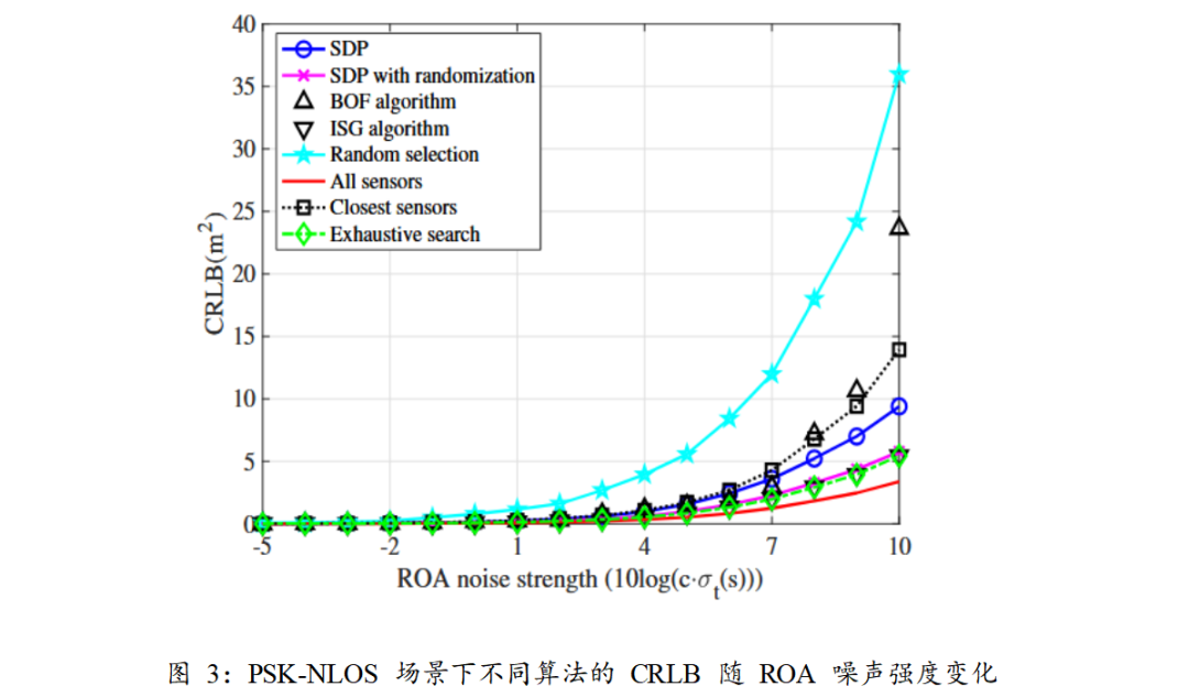 PSU-NLOS Scenario (S=30, K=15, M=10): CRLB changes with different K values: As shown in Figures 5 and 6, when K≤S−M (S−M=20, K=15), both ISG and SDP + randomization algorithms only select LOS sensors, with CRLB=27.2m², 35% lower than random selection (including 5 NLOS); when K>S−M (K=20), the algorithm automatically selects all 15 LOS sensors, with an additional 5 NLOS sensors contributing nothing, and CRLB is basically consistent with K=15 (27.5m²), verifying the conclusion that “only LOS sensors are effective” in the PSU-NLOS scenario.
TotalConclusion
The experiments in this paper show that the impact of reference sensor selection on TDOA accuracy accounts for 40%, and incorrect reference sensors (e.g., those far from the source) can lead to increased CRLB. The dual Boolean vector framework can effectively solve this problem; in the PSK-NLOS scenario, even with 50% of NLOS sensors, using prior information can still improve accuracy by 15% to 20%, providing solutions for NLOS-dominated scenarios such as indoors/rural areas;
However, when sensors move, existing algorithms need to rerun the selection logic (latency), raising questions about whether they can meet high-speed moving scenarios (such as vehicular WSN).
1. Technology Transfer
Introduce Kalman filtering to predict source location, reducing the frequency of selection logic execution; combine AOA/TDOA fusion models, expanding the H matrix to integrate multi-dimensional information, modifying the objective function to “TDOA-CRLB+AOA-CRLB,” enhancing accuracy in complex environments; expand Boolean vector dimensions to K×S (K is the number of sources), constructing a joint CRLB for multiple sources to avoid accuracy degradation caused by interference between sources.
2. Defect Consideration
The research has certain limitations: first, whether this logic can still be applied in moving scenarios; second, the computational complexity is relatively high; third, the existing algorithms do not consider sensor failures, which may lead to increased or decreased CRLB, necessitating the addition of a fault detection module and designing a re-selection mechanism for sensors after failure;
(Master’s Year 2: Junming Kou)

Changchun University of Technology
Laboratory of Safety and Reliability of Complex Systems
END
 END
END z
z


