Research on Pedestrian Recognition Based on Automotive Radar Sensors
Bartsch, A. et al. “Pedestrian recognition using automotive radar sensors.” Advances in Radio Science 10 (2012): 45-55.
1. Introduction and Research Background
The application of automotive radar sensors in pedestrian recognition systems is particularly important because, compared to other systems such as video cameras, radar sensors are significantly less affected by environmental conditions (such as fog, rain, snow, and other adverse weather). In modern vehicles, high-resolution radar sensors have been widely used as part of the Adaptive Cruise Control (ACC) system. If the ACC system and the pedestrian recognition system can share the same radar sensor, the hardware production costs can be kept to a minimum.
This study explores the potential of modern mass-produced automotive radar sensors designed for ACC systems in pedestrian recognition. In particular, the limitations of radar sensors in pedestrian classification decisions are examined to understand what developments future automotive radar sensors need to improve pedestrian recognition systems. The radar-based pedestrian recognition system consists of two main components: the radar sensor and the signal processing unit (i.e., the combination of radar raw data preprocessing and classification algorithms).
2. Analysis of Raw Data from Radar Sensors
2.1 Sensor Technical Parameters
This study used a 77 GHz automotive scanning radar sensor specifically designed for mass-produced ACC systems. The detailed technical characteristics of the sensor are as follows:
| Parameter | Value |
|---|---|
| Frequency Range | 76-77 GHz |
| Doppler Frequency / Radial Relative Velocity Resolution | 390 Hz / 0.77 m/s |
| Azimuth Spatial Discretization | 1° |
| Radial Spatial Discretization | 0.25 m |
| Maximum Detection Distance | 50 m |
| Beam Steering Range (Azimuth) | 17° |
| Beam Width (3 dB, Azimuth) | 2.5° |
| Cycle Time | 66 ms |
| Modulation Technique | Chirp Sequence |
2.2 Data Matrix Structure
The sensor measures the received signal strength values and Doppler shifts for all spatial resolution units every 66 milliseconds. The resolution unit size is 1°×0.25 m. The Doppler shift is proportional to the radial component of the relative velocity between the sensor and the reflecting object, allowing the sensor to easily convert Doppler shift information into radial velocity information. It is important to note that objects moving equidistantly from the sensor do not produce any Doppler shift in the reflected signal.
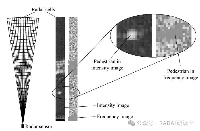
Figure 2 Description: Shows an example of raw radar data for pedestrians. The left side illustrates how the sensor divides its spatial measurement range into resolution units. The sensor measures the power and Doppler shift of the reflected signal in each resolution unit, producing two data matrices: intensity image and frequency image. The gray value of pixels in the intensity image represents the reflected power, while the gray value of pixels in the frequency image corresponds to the measured Doppler shift. A gray value of 128 indicates a Doppler shift of 0 Hz.
In each measurement cycle, a data frame consisting of two matrices is created. The so-called “intensity image” contains the received signal strength values for all spatial resolution units, while the “frequency image” contains the radial relative velocity of the reflection center in each resolution unit. These data matrices constitute the low-level raw radar data used for pedestrian recognition.
3. Pedestrian Recognition Algorithm
3.1 Raw Data Preprocessing
The signal processing chain begins with noise reduction and segmentation in the intensity image. Since simple low-pass filtering can blur the critical boundaries between objects and their surrounding environment, a combination of bit depth reduction and thresholding is employed. The segmentation algorithm creates objects, i.e., spatially adjacent sensor datasets that may originate from the same physical object. This segmentation step significantly impacts classification results as it determines the boundary delineation between objects and noise environments.
In the frequency image, the self-vehicle speed of the measuring vehicle must be compensated. If the vehicle is moving, static objects in front of the vehicle have a relative speed of which is measured by the sensor. Experiments have shown that the vehicle self-speed signal noise generated by the vehicle’s dynamic stability control system is too high for satisfactory compensation. To eliminate this error, known static objects in the radar raw data (e.g., trees or roadblocks identified by another sensor system such as cameras) are needed. Using this information, the frequency image can be compensated with sufficient accuracy for the subsequent recognition process.
3.2 Feature Extraction
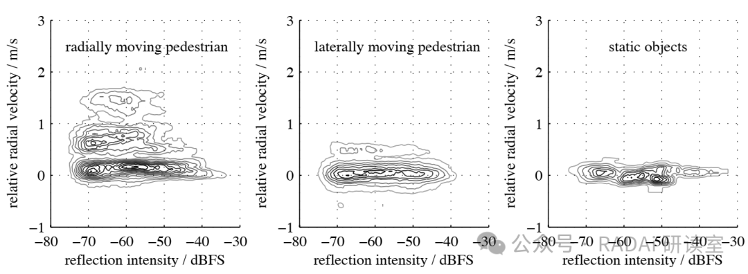
Figure 3 Description: Shows the relative frequency distribution of resolution units with specific reflection intensities and relative radial velocities among different object types. The frequency distribution is retrieved from approximately 150 data frames, with each chart containing about 2000 data points. Since the mean and variance of relative radial velocity values are independent of reflection intensity, the information from the intensity image and frequency image is statistically uncorrelated.
The study proposes a set of five object features that change reliably and significantly when the segmented raw radar data represents pedestrians or static objects. Since pedestrians are radar point targets, their shape in the intensity image is similar to that of any small reflective object. Yamada’s research also indicates that the radar signal intensity reflected by pedestrians, and thus the intensity in the intensity image, is highly variable (approximately 20 dB).
3.2.1 Object Size (Feature m₁)
The object size is a measure proportional to the average radius of the object, simply put, it is the square root of the number of distance-compensated resolution units assigned to the object. Distance compensation is necessary because as the distance from the sensor increases, the received power decreases as and the width of the spatial resolution units increases (since they are always 1° in azimuth). Let be the number of distance-compensated resolution units for the object, the first object feature is:
3.2.2 Object Shape (Feature m₂)
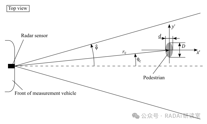
Figure 4 Description: Illustrates the description of the sensor coordinate system, with the object center located at , and the local coordinate system used to calculate the object shape factor. The maximum beam steering angle is the boundary of the azimuth measurement range.
The shape of point targets in radar data is determined by the antenna pattern of the sensor. In the intensity image, small objects have an elliptical shape, with the long axis to short axis ratio in the azimuth direction being approximately . To obtain the shape feature of the object, the difference between the object’s shape and the ideal ellipse is calculated. An ideal ellipse with equal area and semi-axes a, b is placed at the center of the object . In this coordinate system, the i-th resolution unit of the object with units has local coordinates . The distance from the unit to the ellipse boundary is measured as:
where:
The size-normalized cumulative shape error gives the second object feature:
3.2.3 Doppler Spectrum (Features m₃, m₄, m₅)
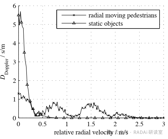
Figure 5 Description: Displays the average Doppler spectrum of radially moving pedestrians and static objects. The Doppler spectrum function is plotted on the relative radial velocity axis v. Since the data is recorded under a non-moving radar sensor, self-vehicle speed compensation is not required.
The Doppler spectrum (DS) is a histogram of the Doppler shift information extracted from all resolution units assigned to the object. It is a density function that indicates the prominence of different relative speeds within the object. The relative radial velocity axis v is divided into small intervals. Resolution units with a radial relative velocity increase the counter for the corresponding interval , where . To obtain the density function, normalization is required such that:
From Figure 5, it is clear that the DS of radially moving pedestrians is wide from 0 to 2.5 m/s. In contrast, the DS of static objects is very narrow, covering only speeds from 0 to 0.4 m/s.
To summarize the shape of the DS into key numbers, consider three intervals . The Doppler spectrum density function integrated over these intervals gives three object features , representing the proportion distribution of radial relative speeds within the object across the three intervals:
where the speed interval boundaries are:. Radial speeds greater than are ignored as they are unlikely to appear in the DS of pedestrians.
3.3 Classification
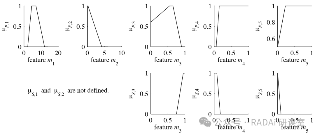
Figure 6 Description: Shows the membership functions and that map the values of object features to the membership values of categories P (pedestrian) and S (static object) and . Note that and are undefined since static objects can be of any shape and size.
The challenge of the classification step is to determine whether an object is a pedestrian or a static object using only the corresponding feature vector . The decision process is based on the knowledge that if an object belongs to a certain category C, certain values of these features are more likely to occur. For example, static objects are unlikely to have significant Doppler information scores in the interval. Therefore, a value of m₃ close to 1 is very unlikely for the “static object” category.
Both valid categories P (pedestrian) and S (static object) have a vector-valued fuzzy membership function , which maps the object’s feature vector m to the corresponding membership value vector of the categories:
close to 1 indicates a high probability for the corresponding category C, while close to zero indicates that the value of m_i is unlikely for that category.
To determine whether category P or S is more suitable for the object, given the fuzzy membership vectors u_P and u_S, the membership vectors are mapped to actual membership values . This is accomplished through a weighted average of the components of the membership vector:
where is the weight vector for category .
Experiments have shown that a constant weight vector is insufficient for correct classification. Instead, the combination of membership values must be closer to logical conjunction. This is achieved by allowing the weight vector to depend on , meaning that lower membership values are weighted more strongly through exponential increase:
Used to increase the base weight is an exponential function chosen empirically. and parameterize this value-dependent weighting, is used to compensate for certain effects when pedestrians have unusual Doppler frequency distributions.
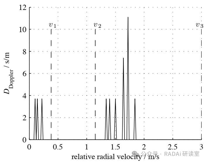
Figure 7 Description: Shows an example of a single-frame Doppler spectrum for a pedestrian. In this case, the object does not contain resolution units with radial relative velocities in the interval. Therefore, the object feature will be zero, as there are some units in the interval, will hold.
4. Experimental Results
4.1 Factors Affecting the Doppler Spectrum
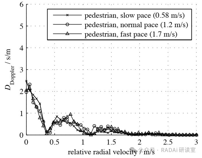
Figure 8 Description: Shows the average Doppler spectrum of walking pedestrians at different walking speeds. In all cases, the motion angle is . Within the investigated walking speed range from to , the DS is independent of the pedestrian’s walking speed.
The DS of walking pedestrians is very stable concerning external influences. It is not affected by the height at which the radar beam hits the person (due to different angles of the antenna beam elevation), as long as sufficient power is reflected for proper segmentation in the intensity image. Additionally, the DS is quite independent of the walking speed of the pedestrian. Walking speeds from to were tested, and they did not affect the DS of the pedestrian, as many different speeds appeared within the segmented object due to arm and leg swings.
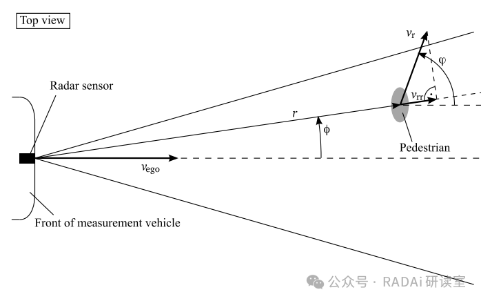
Figure 9 Description: Shows the walking pedestrian with speed relative to the sensor, with a motion angle of , having a radial relative velocity component measurable by the radar sensor.
However, the DS is significantly dependent on the pedestrian’s motion angle. The radar sensor can only measure the radial component of the object’s relative speed. A good approximation is to assume that the pedestrian is centered in front of the sensor, i.e., . Using this approximation, the radial velocity component can be simplified to:
When the motion angle approaches φ = 90°, it approaches zero.
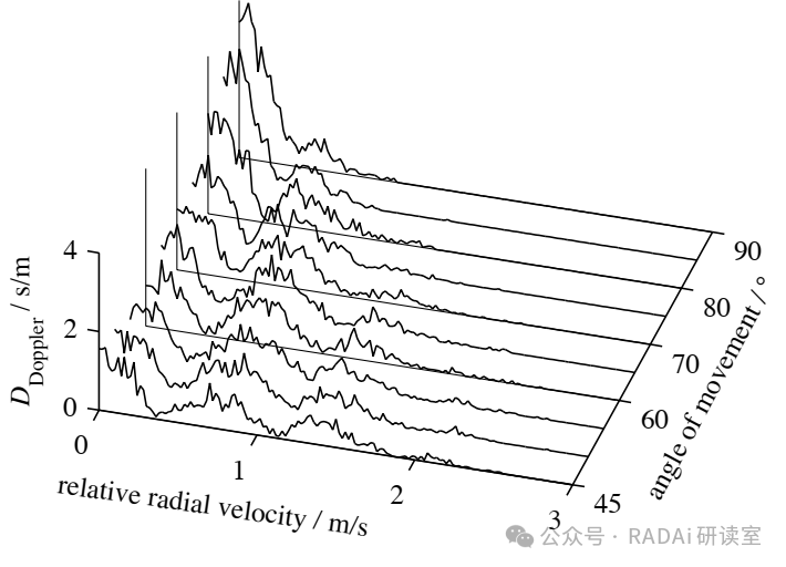
Figure 10 Description: Shows the average Doppler spectrum of walking pedestrians at different motion angles φ. This is a 3D graph showing how the Doppler spectrum changes as the angle increases from 45° to 90°.
Thus, laterally moving pedestrians exhibit a DS very similar to that of static objects. The closer φ is to 90°, the more the DS shows similarity to that of static objects (compare with Figure 5).
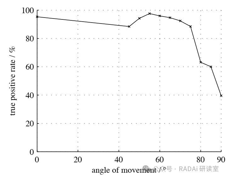
Figure 11 Description: Shows the classification results of walking pedestrians at different motion angles φ. The chart shows that the true positive rate drops from about 95% at φ = 0° to about 40% at φ = 90°.
Thus, the true positive rate after classification reaches 95.3% for radially moving pedestrians (φ = 0°) and drops to 39.5% for laterally moving pedestrians (φ = 90°). Figure 11 shows that when |φ| ≤ 75°, the classification results exceed 88%.
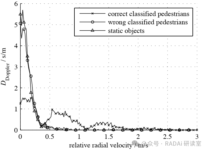
Figure 12 Description: Shows the average Doppler spectrum of correctly classified and misclassified walking pedestrians at various motion angles. The similarity of the Doppler spectrum of misclassified pedestrians and static objects is a limitation of the radar sensor in pedestrian recognition, as in this case the sensor does not provide statistically different data.
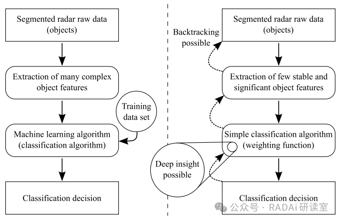
Tracing back from the classification decision to the radar raw data to see whether the sensor data or the classification algorithm is responsible for the misclassified data frames is widely used in empirical optimization of classifiers. As a result, almost all cases where pedestrians were misclassified as static objects can now be traced back to sensor data that even manual inspection cannot distinguish from static object raw data.
4.2 Occluded Pedestrians
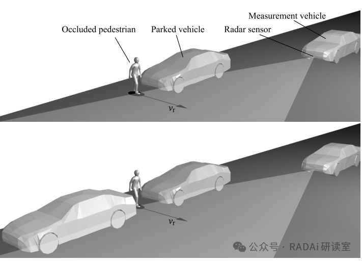
Figure 13 Description: The upper image shows a laterally moving pedestrian occluded by a single parked car. The lower image shows the laterally moving pedestrian now in the gap between two parked cars, where radar waves can propagate due to multiple reflections.
This paper studies two types of occlusion. In the first case, the pedestrian is hidden behind a single parked car; in the second case, the pedestrian is in the gap between two parked cars. In both cases, the pedestrian moves laterally, making them out of the sensor’s line of sight. Lateral movement is a typical characteristic of pedestrians trying to cross the road without looking.
In the case where the pedestrian is in the shadow area behind a parked vehicle at the roadside, the radar waves cannot directly hit the pedestrian. Therefore, the signals reflected by the pedestrian and received by the sensor are very weak. As a result, the pedestrian is blurred with the occluding car, and the segmentation algorithm usually fails to separate the two objects. In the classification step, the true positive rate drops to , which is only slightly better than the false positive rate.
If the pedestrian moves laterally in the gap between two parked cars at the roadside, radar waves can propagate in this gap due to multiple reflections. Therefore, if the gap is not less than 50 cm, the pedestrian will reflect more power to the radar sensor and can be correctly segmented in the radar raw data. Additionally, the recognition results are much better, as the true positive rate rises to 29.4%. This result is significant because the recognition rate is now only 10% lower than that of laterally moving pedestrians in the line of sight.
The recognition results for different gap sizes l are shown in the table below:
| Gap Size l | 30 cm | 50 cm | 70 cm | 90 cm | 110 cm |
|---|---|---|---|---|---|
| r_TP | 20.9% | 29.4% | 28.5% | 20.1% | 25.2% |
| r_FP | 17.6% | 9.5% | 2.4% | 5.4% | 1.4% |
Note that due to segmentation issues in the blurred occlusion area, the false positive rate for narrow gaps (up to 50 cm) is significantly higher.
4.3 False Positives
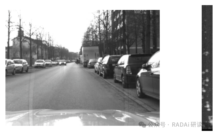
Figure 14 Description: Shows a real urban traffic scene used to measure the false positive rate. The left side is a photo of the scene, and the right side is the corresponding intensity image from the radar raw data.
False positives, i.e., static objects incorrectly classified as pedestrians, result from three fundamental causes. First, the parasitic antenna sidelobe effect may lead to significant scores in the DS of static objects, which appear to have higher speeds than they should. Second, errors in self-vehicle speed compensation may offset the DS. Finally, in cases where errors occur in the segmentation step, resolution units from the object noise environment may be assigned to the object, leading to DS scores that are higher than what is possible for static objects.
To understand how the pedestrian recognition system’s specificity performs in practice, a real urban traffic scene was selected. Vehicles drive along a road with many high-reflective static objects (such as cars) within the measurement range, which is the worst-case scenario for false positives, as high-reflective objects lead to high amplitudes of the antenna sidelobe effect. As a result, a false positive rate of was obtained in the described traffic scene.
4.4 Driving Assistance System Scenarios
The practical use of the pedestrian recognition system described is to avoid collisions by warning the driver of pedestrians moving toward the road, who are occluded in the gaps between parked cars. This scenario includes parked cars as high-reflective static objects, the lateral movement of pedestrians, occlusion, and the linear motion of the measuring vehicle at approximately 8.5 m/s. Under the combination of all these influences in a real scenario, a recognition rate of was achieved. The false positive rate in this specific measurement was .
5. Discussion
The collected results reveal three main areas for future development of radar sensors for pedestrian recognition: Doppler frequency resolution, antenna sidelobes, and spatial resolution.
Doppler Frequency Resolution
For an object located at position , with a relative speed of , the radial velocity component of the object relative to the radar sensor is given by:
(Equation 9 is an approximation of this equation when φ = 0). If the object moves in a straight lateral path (φ = 90°), it still produces a small Doppler shift given by , which has an absolute maximum at the azimuth boundary of the measurement range .
The experimental results described for recognizing laterally walking pedestrians are based on walking speeds of approximately . In this case, the theoretical maximum of the radial relative velocity component is , which is only about one-fifth of the minimum measurable radial speed of 0.77 m/s given by the Doppler frequency measurement resolution of the radar sensor.
However, in experiments, the recognition rate of is much higher than the expected rate of approximately (caused by false positives), even when the pedestrian is centered in front of the sensor (φ = 0), as given by Equation 10. This leads to the conclusion that the micro-Doppler effect (e.g., swinging arms and legs) creates artifacts in the DS, resulting in these classification results.
For specific driving assistance system use cases, it may be necessary to directly measure (without relying on the micro-Doppler effect) the radial velocity component of laterally walking pedestrians within the range of |φ| ≥ 3°, given the walking speed . This requirement gives a blind spot of 5.2 m wide in front of the vehicle at a distance of 50 m. Since this blind spot is usually directly visible, it can be observed by other sensor systems. To meet these requirements, radar sensors with a measurement resolution of at least 0.052 m/s or a Doppler frequency measurement resolution of 26.5 Hz are needed. The required measurement resolution is about 15 times higher than that of the radar sensor used in this paper.
Antenna Sidelobe Effects
The parasitic effects of antenna sidelobes affect the intensity image (ghost targets appear) as well as the frequency image, especially around high-reflective objects. The impact of antenna sidelobes on the intensity image was modeled using the measured antenna pattern. Although this effect can theoretically be compensated, further improvements in the sidelobe performance of today’s radar sensors are needed. Understanding these effects is key to optimizing segmentation algorithms.
Spatial Resolution
If pedestrians are within the line of sight and no more than about 35 m from the sensor, the spatial resolution of the radar sensor is sufficient. However, if pedestrians are occluded by other objects, the corresponding radar data begins to blur with nearby objects. Finer spatial resolution may improve the separability of objects in such cases. If pedestrians are farther from the sensor, the spatial resolution units increase in size because their width is a function of the azimuth. Therefore, distant pedestrians only cover a few resolution units, leading to a DS with very few peaks, which may not well represent the DS. Finer spatial resolution will improve the accuracy of the DS in this regard.
6. Summary and Conclusion
Since pedestrians are point targets for radar sensors, object features from the intensity image cannot be used to distinguish pedestrians from small static objects. Therefore, information from the Doppler frequency image is needed. The Doppler spectrum (a histogram of the measured radial relative speed of the object) has proven to be a stable object feature that contains the information necessary to reliably separate pedestrians from static objects. A simple classification algorithm based on five object features was found to yield classification results comparable to modern machine learning algorithms. Radially moving pedestrians in the line of sight can be recognized with up to 95.3% of samples. The recognition rate for laterally moving pedestrians drops to 39.5%, and for occluded laterally moving pedestrians in the gap between two parked cars, it drops to 29.4%. In cases where pedestrians are misclassified as static objects, the radar sensor does not provide statistically different data from static objects, making it impossible for the classification system (both machine learning and the proposed solution) to determine the correct category using only information from a single radar raw data frame. Therefore, pedestrian recognition using only a single radar raw data frame shows poor classification results.
The main limitations of the radar sensor in this use case have proven to be insufficient Doppler shift measurement resolution and antenna sidelobe effects. It is possible that finer spatial resolution may also improve the sensor’s performance in recognizing occluded pedestrians. Our findings indicate that pedestrian recognition using this low-level approach is limited. Only radar data with higher Doppler frequency measurement resolution (independent of the technology used, such as 24 GHz or 77 GHz) can achieve significant recognition improvements.
Appendix: Mathematical Derivations
A.1 Relationship Between Received Power and Distance
The radar equation describes the relationship between received power and the target distance r. For point targets, the received power is:
where:
- : Transmitted power
- : Transmitting antenna gain
- : Receiving antenna gain
- : Wavelength
- : Radar cross-section (RCS)
- : Target distance
This explains why received power decreases as , which is the theoretical basis for distance compensation.
A.2 Complete Derivation of Doppler Shift
For moving targets, the Doppler shift is given by the following relationship:
where:
- : Radial velocity
- : Wavelength
- : Carrier frequency (77 GHz)
- : Speed of light
For 77 GHz radar:
A.3 Derivation of Radial Velocity Component for Laterally Moving Pedestrians
Consider a pedestrian at position moving with speed and motion angle . The velocity vector of the pedestrian is:
where and are unit vectors in polar coordinates.
The radar can only measure the radial component:
where is the unit vector pointing from the sensor to the target.
After coordinate transformation, we obtain:
When the pedestrian is centered in front of the sensor, it simplifies to:
For pure lateral motion, even if :
This reaches a maximum at the azimuth boundary .
A.4 Detailed Calculation of Elliptical Shape Error
The ideal ellipse equation is:
where the area of the ellipse should equal the area of the object ( resolution units, each with an area of).
Thus:
Given the aspect ratio of the antenna pattern, has , substituting gives:
For the i-th resolution unit located at , the normalized distance to the ellipse boundary is:
When , the unit is outside the ellipse. The cumulative shape error is given by size normalization as feature .
A.5 Design Principles of Fuzzy Membership Functions
The membership function is designed based on Bayesian probability theory. For feature value , the conditional probability for category C is:
The membership value is designed to be proportional to :
where is a normalization constant such that .
A.6 Theoretical Basis for Value-Dependent Weighting
The standard weighted average:
To achieve logical conjunction behavior, when a certain is small, the influence of its weight needs to be increased. The exponential function provides a smooth transition:
When , the weight increase factor approaches ; when , the weight approaches the base weight .
The parameter controls the maximum enhancement factor, while controls the steepness of the transition. Typical values are .
A.7 Quantitative Analysis of Resolution Requirements
For laterally walking pedestrians, it is required to detect the radial velocity component when . Given :
The corresponding Doppler frequency:
The current sensor resolution is 390 Hz (0.77 m/s), thus requiring improvement:
This explains why an improvement of approximately 15 times in resolution is needed.