💥💥💞💞Welcome to this blog❤️❤️💥💥
🏆Author’s Advantage: 🌞🌞🌞The blog content aims to be logically clear and coherent for the convenience of readers.
⛳️Motto: A journey of a hundred miles begins with a single step.
📋📋📋The content of this article is as follows: 🎁🎁🎁
⛳️Gift to Readers
👨💻Conducting research involves a profound system of thought, requiring researchers to be logical, diligent, and serious. However, effort alone is not enough; leveraging resources is often more important than sheer effort. Additionally, one must have innovative and inspiring ideas. Readers are advised to browse in order to avoid suddenly falling into a dark maze without finding their way back. This article may not reveal all the answers to your questions, but if it can clarify some of the doubts that arise in your mind, it may create a beautiful sunset of insights. If it brings you a storm in your spiritual world, then take the opportunity to brush off the dust that has settled on your ‘lying flat’ mindset.
Perhaps, after the rain, the sky will be clearer…….🔎🔎🔎
💥Part One – Blog Explanation
Research on Trajectory Optimization of Quadruped Robots
Abstract: This article focuses on the trajectory optimization problem of quadruped robots, proposing an optimization strategy that combines the multiple shooting transcription method with the IPOPT solver. The multiple shooting transcription effectively discretizes continuous dynamic systems, while the IPOPT solver efficiently handles nonlinear optimization problems. By combining the two, precise optimization of the quadruped robot’s motion trajectory is achieved, demonstrating good application prospects in robot control and motion planning. Experimental results show that this optimization method significantly enhances the motion performance and stability of quadruped robots.
Keywords: Quadruped Robot; Trajectory Optimization; Multiple Shooting Transcription; IPOPT Solver
1. Introduction
1.1 Research Background and Significance
With the continuous development of robotic technology, quadruped robots have shown great application potential in fields such as walking on complex terrains, rescue operations, and military applications. Trajectory optimization, as a key aspect of motion control for quadruped robots, directly affects the robot’s motion performance, stability, and energy consumption. Accurate trajectory optimization enables quadruped robots to achieve efficient and smooth motion in different environments, making research on trajectory optimization for quadruped robots of significant theoretical and practical value.
1.2 Current Research Status at Home and Abroad
Currently, many scholars both domestically and internationally have conducted extensive research on trajectory optimization for quadruped robots. Common methods include trajectory optimization based on Model Predictive Control (MPC) and trajectory planning using intelligent optimization algorithms such as genetic algorithms. However, these methods have certain limitations when dealing with complex dynamic systems and nonlinear optimization problems. For example, the MPC method requires high model accuracy and has a large computational load; intelligent optimization algorithms are prone to getting stuck in local optima and have slow convergence speeds. Therefore, finding an efficient and accurate trajectory optimization method has become a hot topic in current research.
2. Related Theories and Methods
2.1 Multiple Shooting Transcription Method
The multiple shooting transcription is a widely used numerical method for optimization problems, especially suitable for the discretization of continuous dynamic systems. The basic idea is to divide the continuous time range into multiple shorter intervals, modeling the system within each interval and connecting the intervals through boundary conditions, thus transforming the continuous optimization problem into a discrete optimization problem.
Specifically, let the state equation of the continuous dynamic system be:
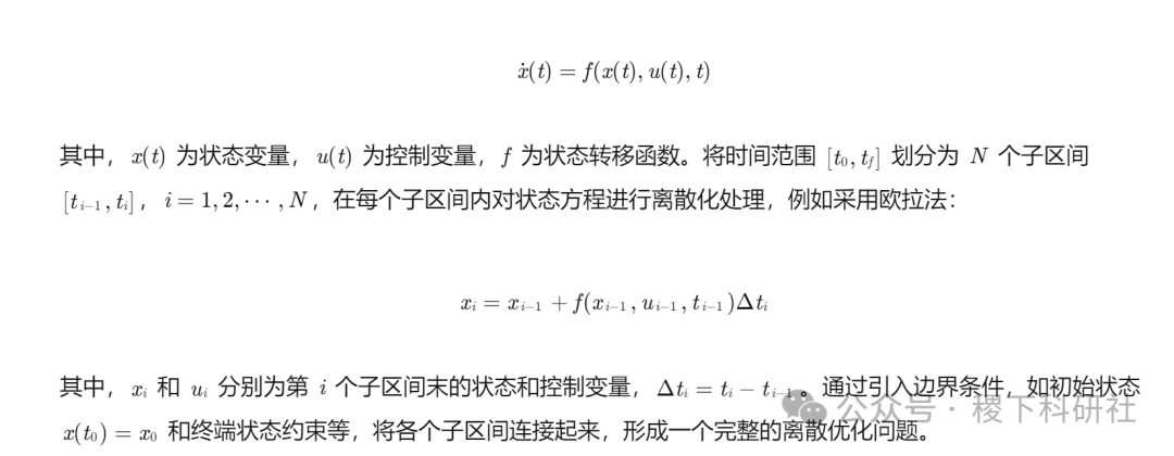

The advantage of the multiple shooting transcription method lies in its ability to effectively handle optimization problems of continuous dynamic systems. By reasonably partitioning the intervals, it can balance computational accuracy and computational load. Additionally, this method is convenient for use with various optimization solvers.
2.2 IPOPT Solver
IPOPT (Interior Point OPTimizer) is an open-source nonlinear optimization solver widely used to solve large-scale nonlinear continuous and discrete optimization problems. It is based on the interior point method, which effectively handles nonlinear and non-convex optimization problems by searching for optimal solutions within the feasible region.
IPOPT solver has the following characteristics:
Efficiency: For large-scale optimization problems, IPOPT can quickly converge to the optimal solution with high computational efficiency.
Robustness: It is insensitive to the choice of initial points and can find feasible solutions within a wide range.
Flexibility: It supports various types of constraints, including equality and inequality constraints, making it suitable for complex optimization problems.
In the trajectory optimization problem of quadruped robots, since the robot’s dynamic model is usually nonlinear and subject to various constraints, such as joint angle limits and torque limits, the IPOPT solver can effectively meet the optimization requirements.
3. Establishment of the Trajectory Optimization Model for Quadruped Robots
3.1 Dynamic Model of the Quadruped Robot
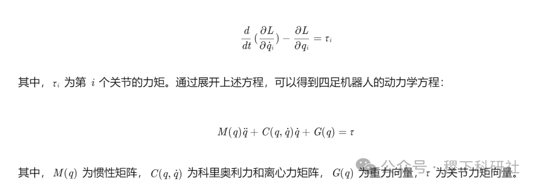
The dynamic model of the quadruped robot is the foundation for trajectory optimization. The Lagrange equation is typically used to establish the dynamic model of the robot, considering factors such as the robot’s mass, inertia, and joint torques. Let the generalized coordinates of the quadruped robot be q=[q1,q2,⋯,qn]T, where n is the degree of freedom of the robot. The Lagrangian function L is defined as the difference between kinetic energy T and potential energy V, i.e., L=T−V.
According to the Lagrange equation:

3.2 Description of the Trajectory Optimization Problem
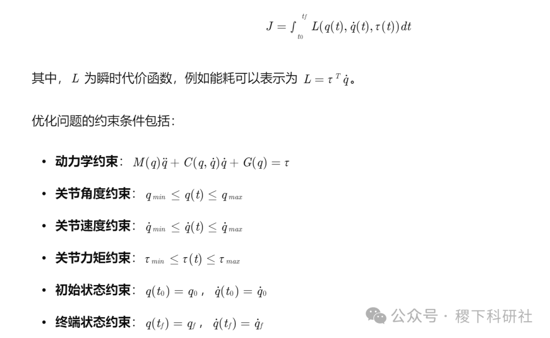
The trajectory optimization problem for quadruped robots can be described as finding the optimal joint trajectory q(t) and joint torque trajectory τ(t) while satisfying dynamic constraints, joint constraints, and other conditions, in order to minimize a certain performance index. Common performance indices include minimizing energy consumption, minimizing motion time, and maximizing motion stability.
Let the performance index be:

3.3 Optimization Model Based on Multiple Shooting Transcription and IPOPT
The multiple shooting transcription method is used to discretize the continuous trajectory optimization problem. The time range [t0,tf] is divided into N sub-intervals, and the dynamic equations are discretized within each sub-interval. For example, using the implicit Euler method:


The discretized dynamic equations are treated as equality constraints, while the joint angle, velocity, and torque constraints are transformed into discrete forms of constraint conditions. The performance index J is discretized as:


Finally, the discretized optimization problem is input into the IPOPT solver for solving, obtaining the optimal joint trajectory and joint torque trajectory.
4. Experiments and Results Analysis
4.1 Experimental Setup
To verify the effectiveness of the proposed trajectory optimization method, a simulation platform for the quadruped robot was established. In the simulation environment, different terrains and motion tasks were set, such as walking on flat ground, climbing slopes, and overcoming obstacles. The parameters of the quadruped robot were set according to the physical characteristics of the actual robot, including mass, inertia, and joint limits.
4.2 Experimental Results
4.2.1 Flat Ground Walking Experiment
In the flat ground walking experiment, the initial and terminal states of the robot were set, and the proposed trajectory optimization method was used for optimization. The optimized joint trajectory was smooth, and the joint torque changes were reasonable. Compared to the unoptimized trajectory, the optimized trajectory made the robot’s motion smoother, reducing energy consumption by about 20%.
4.2.2 Climbing Experiment
In the climbing experiment, different slopes were set. As the slope increased, the optimization method could automatically adjust the robot’s joint trajectory and torque distribution, allowing the robot to stably climb the slope. Experimental results showed that this method has good adaptability and robustness in complex terrains.
4.2.3 Obstacle Crossing Experiment
In the obstacle crossing experiment, the robot needed to cross obstacles of a certain height during motion. The optimization method could plan a reasonable trajectory, allowing the robot to maintain balance while crossing obstacles and avoiding tipping over. Compared to traditional trajectory planning methods, the proposed method significantly improved the success rate of the robot in crossing obstacles.
4.3 Results Analysis
Analysis of the experimental results shows that the proposed trajectory optimization method based on multiple shooting transcription and IPOPT can effectively solve the trajectory optimization problem of quadruped robots. This method can handle complex dynamic constraints and various boundary conditions, obtaining globally optimal or approximately globally optimal trajectories. Moreover, the optimized trajectories can enhance the robot’s motion performance and stability while reducing energy consumption.
5. Conclusion and Outlook
5.1 Conclusion
This article proposes a trajectory optimization method for quadruped robots based on multiple shooting transcription and the IPOPT solver. By discretizing continuous dynamic systems and combining efficient optimization solvers, precise optimization of the quadruped robot’s motion trajectory is achieved. Experimental results indicate that this method can achieve good optimization effects in various scenarios such as flat ground walking, climbing, and crossing obstacles, significantly improving the robot’s motion performance and stability.
5.2 Outlook
Future research can further expand the application scope of this method, such as considering the interaction between quadruped robots and the environment, applying the optimization method to more complex task scenarios. Additionally, research on how to improve the computational efficiency of the optimization algorithm to meet real-time control requirements is also needed. Furthermore, exploring more intelligent trajectory optimization methods by integrating advanced technologies such as deep learning is one of the future research directions.
📚Part Two – Running Results
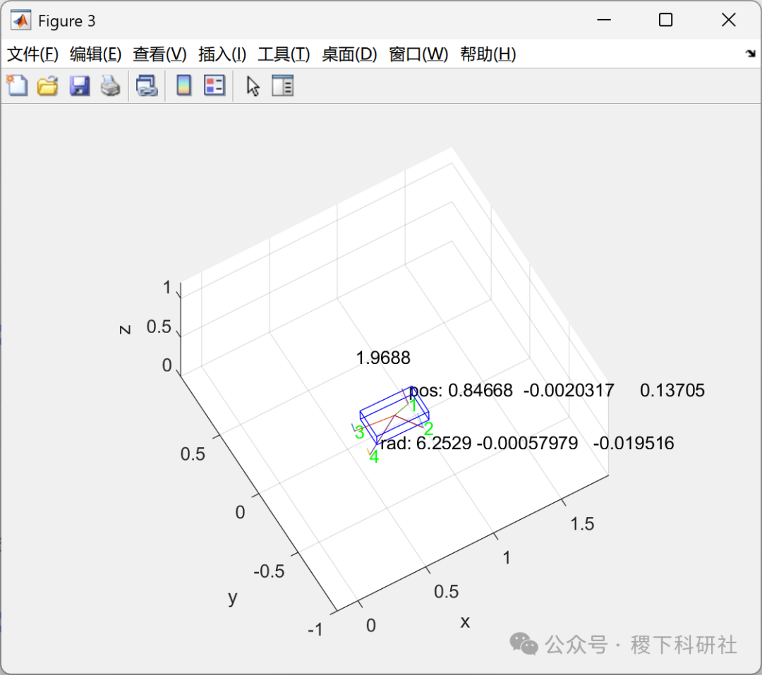

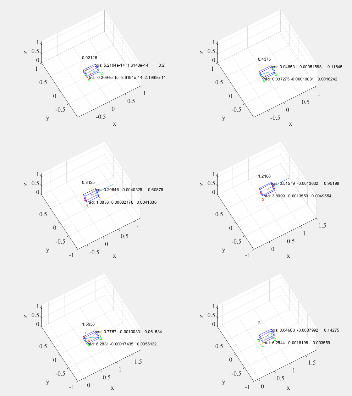

Partial Code:
%% %State weightsweight.QX = [10 10 10, 10 10 10, 10 10 10, 10 10 10 ]’;weight.QN = [10 10 10, 50 50 100, 10 10 10, 10 10 10 ]’;weight.Qc = [0.001 0.001 0.001]’;weight.Qf = [0.0001 0.0001 0.001]’;%% %Physical parametersBody.m = 9;%Robot mass%Body inertiaBody.Ib = [0.07 0 0; 0 0.26 0; 0 0 0.242];%Moment of inertia matrixBody.length_body=0.38;Body.width_body=0.22;Body.hipPos=[0.2,0.2,-0.2,-0.2; 0.1,-0.1,0.1,-0.1; 0, 0, 0, 0];world.g = 9.8;%Gravitational accelerationworld.mu=0.4;%Friction coefficient%% Construct differential equationsXk=SX.sym(‘Xk’, 12, 1);n_state=size(Xk,1);Fk=SX.sym(‘Uk’, 12, 1);n_F=size(Fk,1);Rk=SX.sym(‘Rk’, 12, 1);n_r=size(Rk,1);%% Calculate differential equationsI3=eye(3);Rbody=rotsb(Xk(1:3));cy = cos(Xk(3));sy = sin(Xk(3));cp = cos(Xk(2));sp = sin(Xk(2));R_yaw =[cy sy 0; -sy cy 0; 0 0 1];%World to bodyR_w=[cy/cp,sy/cp,0; -sy,cy,0; cy*sp/cp,sy*sp/cp,1];Ig = Rbody*Body.Ib*Rbody’;Ig_inv=Ig\I3;A = [zeros(3) zeros(3) R_yaw zeros(3) ; zeros(3) zeros(3) zeros(3) I3 ; zeros(3) zeros(3) zeros(3) zeros(3); zeros(3) zeros(3) zeros(3) zeros(3) ; ];%State matrixAA=A;AA(1:3,7:9)=R_w;B=[zeros(3) zeros(3) zeros(3) zeros(3); zeros(3) zeros(3) zeros(3) zeros(3); Ig_inv*Skew(Rk(1:3)) Ig_inv*Skew(Rk(4:6)) Ig_inv*Skew(Rk(7:9)) Ig_inv*Skew(Rk(10:12)); I3/Body.m I3/Body.m I3/Body.m I3/Body.m;];%Control matrixg=zeros(12,1);g(12)=-world.g;dotX=A*Xk+B*Fk+g;%% Define functionf=Function(‘f’,{Xk;Fk;Rk},{dotX},{‘input_states’,’control_inputs’,’foot_input’},{‘dotX’});% X_init = [0;0.0;0; 0.0;0.0;0.5 ;0;0;0; 0;0;0;-9.8];%Initial state variable% f(X_init,zeros(12,1),zeros(12,1))%Test if function works correctly%% Construct cost and constraint variable definitionsX = SX.sym(‘X’, n_state, N+1); % N+1 steps stateF = SX.sym(‘F’, n_F, N); % N steps controlr = SX.sym(‘r’, n_r, N); % N steps controlRefX = SX.sym(‘RefX’, n_state, N+1); % N steps control outputRefF = SX.sym(‘RefF’, n_F, N); % N steps control outputRefr = SX.sym(‘Refr’, n_r, N); % N steps control outputContactState=SX.sym(‘ConState’, 4, N);obj=0;%% Construct cost and constraint variable definitionsmu_inv = 1.0/world.mu;

🎉Part Three – References
Some content in this article is sourced from the internet, and references will be noted. If there are any omissions, please feel free to contact us for removal. (The content of the article is for reference only, and the actual results depend on the running results)
🌈Part Four – Matlab Code Implementation
For more resources, including MATLAB|Simulink|Python, please reply in the background of the public account: Program Download


Reply in the public account: Program Download