This code implements a positioning system based on geomagnetic feature matching, using the Extended Kalman Filter (EKF) for loosely coupled fusion, combining geomagnetic observation data with Inertial Measurement Unit (IMU) data to achieve high-precision carrier positioning.

Table of Contents

• Program Overview
• System Overview
• Core Technical Features
• System Architecture Process
• Simulation Scenario Design
• Core Algorithm Module
• Performance Evaluation Metrics
• Operating Results
• MATLAB Source Code

Program Overview

System Overview

This code implements a positioning system based on geomagnetic feature matching, using the Extended Kalman Filter (EKF) for loosely coupled fusion, combining geomagnetic observation data with Inertial Measurement Unit (IMU) data to achieve high-precision carrier positioning.

Core Technical Features

Geomagnetic Matching Positioning Technology:

• Principle: Utilizing the spatial distribution characteristics of the Earth’s magnetic field, position estimation is performed by matching real-time magnetic field measurements with pre-stored geomagnetic maps.
• Advantages: Does not rely on external signal sources, has good anti-interference capability and concealment.
• Application Scenarios: Suitable for environments where GPS signals are limited, such as indoors, underground, underwater, etc.

Loosely Coupled Fusion Architecture:

• Geomagnetic System: Provides absolute position information but has a lower update frequency and limited accuracy.
• Inertial Navigation System: Provides continuous motion state estimation but has cumulative errors.
• Fusion Strategy: Uses EKF to complement the advantages of both systems, achieving continuous high-precision positioning.

System Architecture Process

Phase One: Independent Geomagnetic Positioning

1. Geomagnetic Map Generation: Construct a reference map containing the spatial distribution of magnetic field intensity.
2. Feature Matching: Calculate similarity between real-time magnetic field measurements and the map.
3. Position Estimation: Select the position with the highest similarity as the geomagnetic positioning result.

Phase Two: EKF Loosely Coupled Fusion

1. Prediction Step: Predict the current state based on IMU acceleration data and motion model.
2. Update Step: Use the geomagnetic positioning result to correct the predicted state.
3. Optimal Estimation: Output the fused optimal position and velocity estimates.

Simulation Scenario Design

Motion Trajectory:

• Trajectory Type: Circular motion trajectory.

• Parameter Settings:

• Center Position: (50, 50)
• Radius: 20 meters
• Angular Velocity: 0.1 rad/s
• Simulation Time: 50 seconds

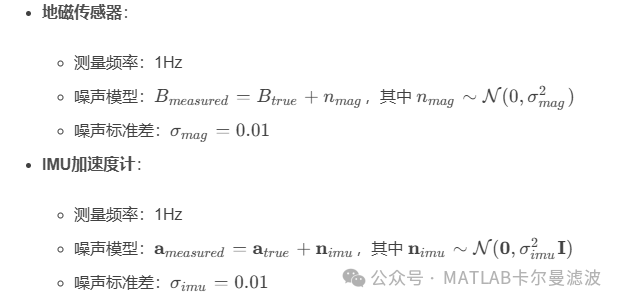
• Geomagnetic Sensor:

• Measurement Frequency: 1Hz

Core Algorithm Module

Geomagnetic Feature Matching Algorithm:

% Similarity Calculation (Negative Relative Error)
similarity(i,j)=-abs(measurement - mapValue)/ mapValue

EKF State Estimation:

• State Vector: [x, y, vx, vy]ᵀ (position and velocity)
• Motion Model: Constant velocity model + acceleration control input
• Observation Model: Direct observation of position coordinates

Covariance Matrix Design:

• Process Noise: Consider the uncertainty of IMU integration.
• Observation Noise: Distinguish the different accuracy characteristics of geomagnetic observations and IMU observations.

Performance Evaluation Metrics

Positioning Accuracy Metrics:

• Average Positioning Error
• Maximum Positioning Error
• Final Position Error
• Error Cumulative Distribution Function (CDF)

System Comparative Analysis:

• Independent Geomagnetic Positioning vs EKF Fusion Positioning
• Pure Inertial Navigation vs Fusion Navigation
• Quantitative Analysis of Improvement Effects

Operating Results

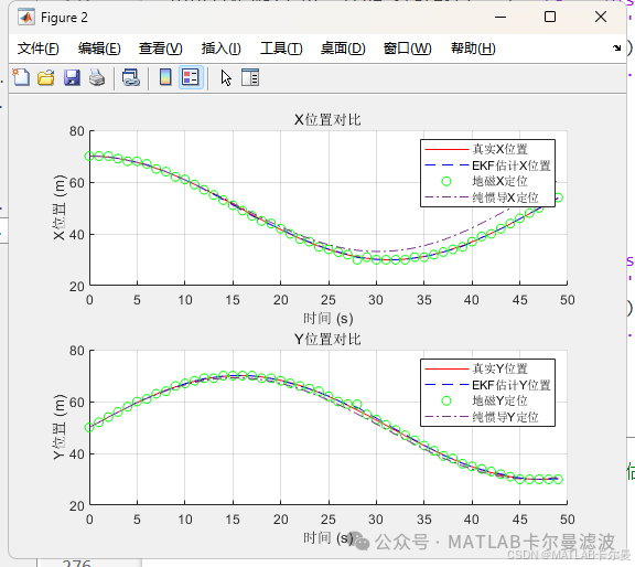
Trajectory and Fusion Error Comparison: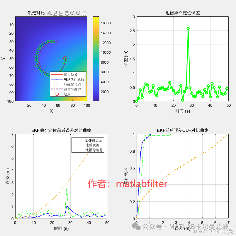Position Comparison Curves for Each Axis:Command Line Output Results: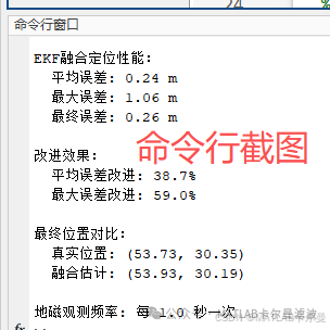Program Structure: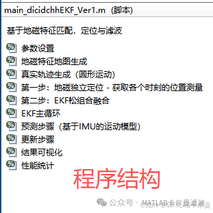

MATLAB Source Code

Partial code is as follows:

% Based on geomagnetic feature matching, positioning and filtering
% For paid consultation or customization, please contact V: matlabfilter (only this one, others are pirated stores)
% 2025-09-14/Ver1

clear; clc; close all;
rng(0);

%% Parameter Settings
dt =1;% Time step (s)
T =50;% Total simulation time (s)
N = T / dt;% Total steps

mapSize =100;% Map size
noiseLevel_mag =0.01;% Geomagnetic noise intensity
noiseLevel_imu =0.01;% IMU noise intensity
mag_measurement_freq =1;% Geomagnetic measurement frequency: measure once every step

%% Geomagnetic Feature Map Generation
Bx =rand(mapSize, mapSize)*10+[1:mapSize]'*[1:mapSize];
By =rand(mapSize, mapSize)*30+[1:mapSize]'*[1:mapSize];
Bz =rand(mapSize, mapSize)*50+[1:mapSize]'*[1:mapSize];
m_magneticMap =sqrt(Bx.^2+ By.^2+ Bz.^2);% Magnetic field intensity distribution

%% True Trajectory Generation (Circular Motion)
center =[50,50];
radius =20;

Complete code download link:

https://mall.bilibili.com/neul-next/detailuniversal/detail.html?isMerchant=1&page=detailuniversal_detail&saleType=10&itemsId=13156396&loadingShow=1&noTitleBar=1&msource=merchant_share

Or click on “Read the original text” at the end to jump.

<span>If you need help or have customization requirements related to navigation and positioning filtering, please contact the author via WeChat below.</span>