
Explanation of Analytical Solution
A cantilever plate with three free edges and one fixed edge can solve the variational equation by reducing it to a regular ordinary differential equation in another direction using one-way analytical methods.
Analytical Solution Process: For specifics, please refer to Cao Zhiyuan’s “Theory of Plate and Shell Vibrations” pages 47-49.
Finite Element Method Solution
ANSYS Solution:
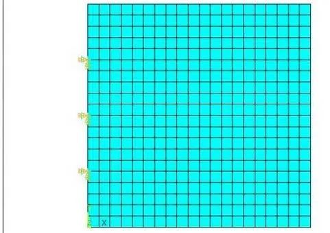
Taking a square cantilever plate with a length and width of 2 as an example:
Material Parameters: Elastic Modulus E=2.1e11, Poisson’s ratio g=0.3, Density r=7.3e3, Thickness t=0.05
Mesh Division: Divide into 20 elements in both length and width directions (to be consistent with the subsequent program)
/PREP7
BLC4, , ,2,2
! Preprocessing: Draw a 2×2 rectangle
MP,DENS,1,7.3e3
! Density
MP,EX,1,2.1e11
! Elastic Modulus
MP,PRXY,1,0.3
! Poisson’s Ratio
ET,1,SHELL63
! Element Type
R,1,0.05,0.05,0.05,0.05,, ,
! Real Constants, Thickness
TYPE,1 MAT,1REAL,1
! Material and Element Type Number
ESIZE,0.1,0,
! Element length of 0.1
AMESH,all
! Draw Mesh
DL,4,,ALL,
! Apply Fixed Constraint
FINISH
! Direct Solve Command Stream! Overall Solve
/SOL
ANTYPE,2
MODOPT,LANB,10
EQSLV,SPAR
MODOPT,LANB,20,0,99999999, ,OFF
SOLVE
Table 1 ANSYS Direct Solve Results

The above references Xu Bin, Gao Yuefei, and Yu Long’s “Dynamic Analysis and Engineering Applications of Finite Element in MATLAB”.
Finite Element Method to Solve Cantilever Plate Modal MATLAB Program:
Does not include subfunctions for calculating element stiffness and mass
clear all
clc
% Clear Variables
tic
% Start Timing
% Define Material
E=2.1e11;
% Elastic Modulus
poisson =0.3;
% Poisson’s Ratio
density=7.3e3;
% Density
t=0.05;
% Plate Thickness
lx=2;
% Length in x direction
ly=2;
% Length in y direction
jdx=21;
% Number of nodes in x direction
jdy=21;
% Number of nodes in y direction
% Initialization
% Stiffness and Mass Matrix
Tol_dof=3*jdx*(jdy-1);
% Apply fixed constraints on y=0 boundary, remove 21 nodes
k(1:Tol_dof,1:Tol_dof)=0;
% Total Stiffness Matrix
m(1:Tol_dof,1:Tol_dof)=0;
% Total Mass Matrix
Tol_element=(jdx-1)*(jdy-1);
% Total Number of Elements
% Node Matrix
en(1:Tol_element,1:4)=0;
% Each element has four nodes, record node numbers
for ni=1:jdx-1
for nj=1:jdy-1
en(ni+(nj-1)*(jdx-1),1)=ni+(nj-1)*jdx;
en(ni+(nj-1)*(jdx-1),2)=ni+1+(nj-1)*jdx;
en(ni+(nj-1)*(jdx-1),4)=ni+nj*jdx;
en(ni+(nj-1)*(jdx-1),3)=ni+1+nj*jdx;
end
end
% Node Displacement, Constraints, and Degree of Freedom Coordinates
disp(1:jdx*jdy,1:3)=1;
% Displacement Matrix
constraints=1:1:jdx;
% Constrained Nodes on y=0
disp(constraints,:)=0;
dof=0;
% Degree of Freedom Marking
for ni=1:jdx*jdy
for nj=1:3
if disp(ni,nj)~=0
% No numbering for constrained
dof=dof+1;
disp(ni,nj)=dof;
end
end
end
% Element Length
el=lx/(jdx-1);
eh=ly/(jdy-1);
% Four-node 12-degree of freedom Element Stiffness and Mass Matrix
% Input Material Parameters and Node Concentrated Length
[ek,dm]=km(el/2,eh/2,poisson,t,E,density);
% Global Stiffness Matrix and Mass Matrix
tg(1:12)=0;
% Mark, Element Matrix Dimension
forloopi=1:(jdx-1)*(jdy-1)
% Outer Loop, Elements
for zi=1:4
% Each Node has Three Degrees of Freedom
tg((zi-1)*3+1)=disp(en(loopi,zi),1);
tg((zi-1)*3+2)=disp(en(loopi,zi),2);
tg((zi-1)*3+3)=disp(en(loopi,zi),3);
end
for jx=1:12
for jy=1:12
if(tg(jx)*tg(jy)~=0)
k(tg(jx),tg(jy))=k(tg(jx),tg(jy))+ek(jx,jy);
m(tg(jx),tg(jy))=m(tg(jx),tg(jy))+dm(jx,jy);
end
end
end
% Total Stiffness and Mass Matrix
end
% Solve Eigenvalue Problem
[v,d] = eig(k,m);
% eig function solves eigenvalue problem
tempd=diag(d);
% Record Eigenvalues
[nd,sortindex]=sort(tempd);
% Sort Eigenvalues
v=v(:,sortindex);
% Sort Eigenvectors
mode_number=1:15;
% Solve Order
frequency(mode_number)=sqrt(nd(mode_number))/(2*pi);
% Record Angular Frequency
toc% End Timing
Table 2 MATLAB Direct Solve Results
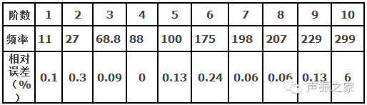
The tenth order frequency differs significantly; extracting the mode shape analysis from the ANSYS analysis, it can be seen that the tenth frequency corresponds to the bending mode parallel to the fixed edge. This direction does not include degrees of freedom in the thin plate bending element, thus taking the eleventh frequency from the ANSYS analysis, which is 300.1Hz. Compared to the MATLAB result, the error is 0.29%.
Using Modal Synthesis Method to Solve
The basic principle of the modal synthesis method can be referenced in Liu Mingjie’s article “Dynamics Principles of Fixed Interface Modal Synthesis,” published in the June 1985 issue of the Journal of Zhejiang University (Engineering Edition).
The core of the modal synthesis method is two coordinate transformations, explained clearly in the paper:
First Coordinate Transformation: The modal matrix reduces the stiffness and mass matrices of each substructure;
Second Coordinate Transformation: The displacements at the nodes at the interface must be equal, achieving the coupling between substructures.
ANSYS Modal Synthesis Method Solution
ANSYS modal synthesis method is applied in dynamic analysis of substructures, and its basic process includes three aspects: generation process, use process, and extension process. ANSYS provides a user-friendly modal synthesis (Component Mode Synthesis) CMS wizard (Preprocessor>Modeling>CMS) that allows easy definition of super-elements and interfaces, and management and organization of files generated by modal synthesis analysis.
1. Create super-elements
2. Select CMS solving method (CMSOPT): fixed interface method or free interface method.
3. Name super-element matrix file (SEOPT).
4. When considering damping, input concentrated mass matrix formula.
5. Define primary degrees of freedom: define primary degrees of freedom at the interface of the super-elements.
6. Maintain database: This is necessary because the same database file is needed when extending modes.
7. Solve to generate super-element matrix file.
The usage and extension part of CMS is basically the same as for substructures, but CMS only supports modal analysis. In substructure analysis, each substructure in the overall structure needs to be generated and extended, and then each substructure is combined into the entire model. In the free interface modal synthesis method, the number of modal modes to be extended using MODOPT should be less than the number of modal modes solved for each super-element. If more modes need to be extended, the CMS super-element needs to be re-solved for more orders.
Continuing the analysis with the example from the first floor:
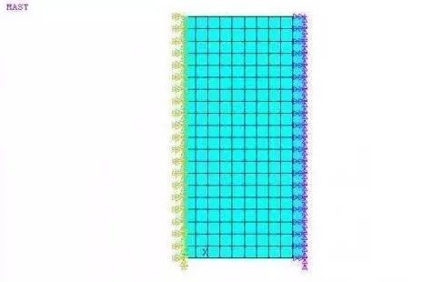
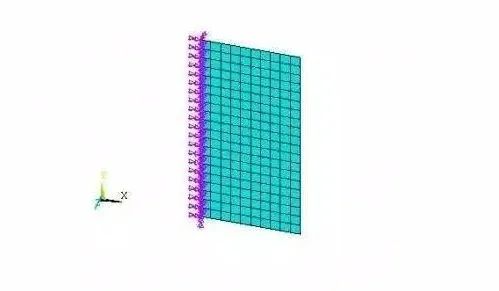
It is necessary to first establish three sets, two element sets and one interface node set; writing it as an APDL command stream is more cumbersome than using GUI operations.
Substructure A:
/filnam,part1
! File Name part1 Substructure A
/solu antype,substr
! Analysis Type Substructure
seopt,part1,2
! Substructure A
cmsopt,fix,20
! Fixed Interface Method to Solve for the First 20 Frequencies
cmsel,s,part1
! Select part1 element set
cmsel,s,interface
! interface node set
m,all,all
! Select All
nsle solve finish save
! Solve and Save
Substructure B:
/filnam,part2
! File Name part2 Substructure B
/solu antype,substr
! Analysis Type Substructure
seopt,part2,2
! Substructure B
cmsopt,fix,20
! Fixed Interface Method to Solve for the First 20 Frequencies
cmsel,s,part2
! Select part2 element set
cmsel,s,interface
! interface node set
m,all,all
! Select All
nsle solve finish save
! Solve and Save
Fixed Interface Modal Synthesis Method Solve Command Stream:
/clear,nostart
! Clear Variables, Start a New Analysis
/filnam,use
! File Name use Overall Structure
/prep7
et,1,matrix50
! Define Super-element
type,1
se,part1
! Select Substructure One
se,part2
! Select Substructure Two
finish
/solu
antype,modal
! Analysis Type
modopt,lanb,10
! Solve for the First 10 Frequencies
solve
finish
save
Table 3 ANSYS Modal Synthesis Method Solve Results
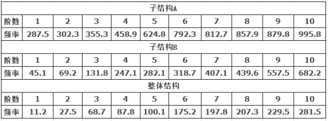
Comparing with the directly solved structure in Table 1, it can be seen that in this case, the ANSYS modal synthesis method has higher accuracy (retaining one decimal place), and the first 10 frequencies are basically consistent. In calculating large complex structures, the modal synthesis method can save a large amount of computation time and computer resources, improving efficiency; at the same time, it allows flexible modification of the design of large systems’ subsystems. Therefore, for complex large structures such as airplanes, vehicles, ships, and high-rise buildings, using the ANSYS modal synthesis method for modal analysis can provide better solutions in terms of accuracy and computational speed.
Main Modal Analysis MATLAB Program:
The division of substructures is consistent with the handling in ANSYS, as follows:
Substructure A (only listing modified parts):
lx=2;
% Length in x direction
ly=1;
% Length in y direction
jdx=21; % Number of nodes in x direction
jdy=11; % Number of nodes in y direction
% y=0 and 1 along the x-axis remove 42 points to obtain total degrees of freedom
Tol_dof=3*jdx*(jdy-2);
cons_Ori=1:1:jdx;
% Original Constrained Nodes
% For fixed interface method, apply constraints
cons_Arti=jdx*(jdy-1)+1:1:jdx*jdy;
% Total Constraints
constraints=[cons_Ori,cons_Arti];
master_mode=15;
add_num=jdx*3;
% Take the first master_mode orders as modal synthesis
fi_unres1=cat(1,v(1:master_mode,:)’,zeros(add_num,master_mode));
Substructure B (only listing modified parts):
lx=2;
% Length in x direction
ly=1;
% Length in y direction
jdx=21;
% Number of nodes in x direction
jdy=11;
% Number of nodes in y direction
% Total Degrees of Freedom
Tol_dof=3*jdx*(jdy-1);
% For fixed interface method, apply constraints
cons_Arti=1:1:jdx;
% Single-sided constrained node numbers
constraints=cons_Arti;
% Total Constraints
master_mode=15;
add_num=jdx*3;
fi_unres2=cat(1,zeros(add_num,master_mode),v(1:master_mode,:)’);
% In the main modal, it is assumed that the nodes with fixed constraints have zero displacement, and are supplemented to complete the modal synthesis
Table 4 MATLAB Substructure Solve Results
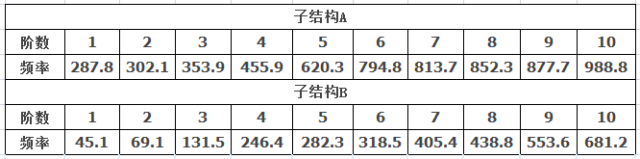
Constrained Modal Analysis Program as follows:
Substructure One (only listing modified parts):
lx=2;
% Length in x direction
ly=1;
% Length in y direction
jdx=21;
% Number of nodes in x direction
jdy=11;
% Number of nodes in y direction
Tol_dof=3*jdx*(jdy-1);
cons_Ori=1:1:jdx;
% Original Constrained Nodes
constraints=cons_Ori;
% Total Constraints
% In the total stiffness matrix, block by whether on the interface
add_num=jdx*3;
master_mode=15;
kii=k(1:end-add_num,1:end-add_num);
kij=k(1:end-add_num,end-add_num+1:end);
% Extract Constrained Modal
fi_res1=cat(1,-inv(kii)*kij,eye(add_num));
% Merge Total Modal
fi_1=cat(2,fi_unres1,fi_res1);
% Use Modal to Perform First Coordinate Transformation on Stiffness and Mass Matrix
k1=fi_1’*k*fi_1; m1=fi_1’*m*fi_1;
Substructure Two (only listing modified parts):
lx=2;
% Length in x direction
ly=1;
% Length in y direction
jdx=21;
% Number of nodes in x direction
jdy=11;
% Number of nodes in y direction
% Total Degrees of Freedom
Tol_dof=3*jdx*jdy;
% Substructure has no constraints
% In the total stiffness matrix, block by whether on the interface
add_num=jdx*3;
master_mode=15;
kii=k(add_num+1:end,add_num+1:end);
kij=k(add_num+1:end,1:add_num);
% Extract Constrained Modal
fi_res2=cat(1,eye(add_num),-inv(kii)*kij);
% Merge Total Modal
fi_2=cat(2,fi_res2,fi_unres2);
% Use Modal to Perform First Coordinate Transformation on Stiffness and Mass Matrix
k2=fi_2’*k*fi_2;
m2=fi_2’*m*fi_2;
Modal Synthesis Program as follows:
master_mode=15;
% master_mode is the order to retain for the main modal
add_num=jdx*3;
% add_num is the number of degrees of freedom on the interface
Tol_num=length(k1);
% Tol_num is the dimension of the transformed stiffness matrix
K=zeros(2*Tol_num);
M=zeros(2*Tol_num);
% Initialize Modal Synthesis Matrix
K(1:Tol_num,1:Tol_num)=k1;
K(Tol_num+1:end,Tol_num+1:end)=k2;
M(1:Tol_num,1:Tol_num)=m1;
M(Tol_num+1:end,Tol_num+1:end)=m2;
% Non-coupled modal synthesis matrix, directly written in matrix form
beta=zeros(2*Tol_num,2*master_mode+add_num);
beta(1:master_mode,1:master_mode)=eye(master_mode);
beta(master_mode+1:master_mode+add_num,master_mode+1:master_mode+add_num)=eye(add_num);
beta(master_mode+1+add_num:master_mode+2*add_num,master_mode+1:master_mode+add_num)=eye(add_num);
beta(end-master_mode+1:end,end-master_mode+1:end)=eye(master_mode);
% The second coordinate transformation matrix beta, easily obtainable from displacement columns
KK=beta’*K*beta;
MM=beta’*M*beta;
% Perform Second Coordinate Transformation
[v,d] = eig(KK,MM);
tempd=diag(d);
[nd,sortindex]=sort(tempd);
v=v(:,sortindex);
% Solve Eigenvalue Problem
mode_number=1:5;
frequency_sum(mode_number)=sqrt(nd(mode_number))/(2*pi);
% Obtain final frequencies from the modal synthesis method
Table 5 MATLAB Modal Synthesis Method Solve Results

The results from MATLAB are not very good; only the fundamental frequency is acceptable. It is unclear whether this is due to the fixed interface modal synthesis method itself or the program’s issues.
. 2023 Annual Plan Query
- Method 1: Scan the QR code below with WeChat to enter the page

- Method 2: 18510898133 (WeChat) Manager Li
Welcome to Forward
 Click to Share
 Click to Collect
 Click to Like
 Click to View