💥💥💞💞Welcome to this blog❤️❤️💥💥
🏆Author’s Advantages:🌞🌞🌞The blog content aims to be logically coherent and clear for the convenience of readers.
⛳️Motto:Those who travel a hundred miles should consider ninety as half.
💥1 Overview
Image data is indispensable in daily communication and interaction. However, during transmission and reception, images are often interfered with by noise due to hardware devices, which can degrade image quality and affect subsequent processing and analysis. Therefore, removing image noise is crucial. Currently, how to remove noise while preserving the texture details of the image remains a pressing issue. In recent years, the rise of sparse representation theory has led to significant breakthroughs in image denoising.
Image denoising is an important research topic in the fields of image processing and computer vision, aiming to recover a clear original image from noise-polluted images. Sparse constraint-based image denoising algorithms have received widespread attention in recent years because they can effectively remove noise while preserving image details and structure.
Research on Image Denoising Algorithm Based on Sparse Constraints
Abstract
The sparse constraint-based image denoising algorithm is based on the assumption that images have sparsity in a specific transform domain. By using techniques such as sparse coding and dictionary learning, it effectively removes noise while retaining image details. This paper reviews the theoretical foundations, key technologies, typical algorithms, and their advantages and challenges in sparse constraint image denoising, and looks forward to future research directions.
1. Introduction
Image denoising is a significant task in the field of digital image processing, aimed at removing noise from images to improve image quality and provide a foundation for subsequent processing (such as segmentation, recognition, etc.). Traditional denoising methods (such as filtering, statistical modeling, etc.) often struggle to effectively distinguish between noise and image details, leading to image blurring or introducing artifacts. In recent years, sparse constraint-based image denoising algorithms have gained widespread attention due to their excellent denoising performance and good preservation of image details.
2. Theoretical Foundation of Sparse Representation
The theory of sparse representation posits that natural images exhibit sparsity in appropriate transform domains (such as wavelet transform, Fourier transform, or dictionary learning), meaning that most of the image’s energy is concentrated in a few coefficients, while the remaining coefficients are close to zero. This theory provides a new approach for image denoising: by finding the sparse representation of the image in a certain transform domain, suppressing or removing noise coefficients, and then reconstructing the image to achieve denoising.
3. Key Technologies
Sparse constraint-based image denoising algorithms typically include the following key steps:
3.1 Image Block Division
Divide the noisy image into several overlapping or non-overlapping image blocks, treating each block as an independent sample. This block division strategy can effectively utilize the local structural information of the image, improving algorithm efficiency.
3.2 Sparse Coding
For each image block, find its sparse representation in the selected transform domain. This is usually an optimization problem aimed at minimizing reconstruction error while constraining the sparsity of the coefficients. Common methods include:
- L0 Norm: Directly constrains the number of non-zero coefficients, but this is a non-convex optimization problem that is difficult to solve.
- L1 Norm: The optimal convex approximation of the L0 norm, effectively inducing sparsity, and can be solved using various optimization algorithms, such as Iterative Soft Thresholding Algorithm (ISTA) and Alternating Direction Method of Multipliers (ADMM).
3.3 Coefficient Thresholding
Process the sparse representation coefficients based on threshold criteria to suppress or remove noise coefficients. Common threshold criteria include:
- Hard Threshold: Sets coefficients with absolute values less than the threshold to zero, retaining coefficients with absolute values greater than the threshold.
- Soft Threshold: Sets coefficients with absolute values less than the threshold to zero and shrinks coefficients with absolute values greater than the threshold.
3.4 Image Reconstruction
Reconstruct the image blocks using the processed sparse coefficients, and then stitch all reconstructed image blocks together to form the denoised image. Since there is overlap between image blocks, averaging or weighted averaging strategies are needed to eliminate stitching artifacts.
4. Typical Algorithms
4.1 K-SVD Algorithm
K-SVD is a dictionary learning-based image denoising algorithm. It alternately iterates to update the dictionary and sparse coefficients, finding a dictionary that adapts to the image features, achieving better denoising results.
4.2 BM3D Algorithm
BM3D (Block-Matching and 3D Filtering) combines non-local similarity and sparse representation ideas. It first searches for image blocks similar to the current block, stacks them into a three-dimensional matrix, performs sparse coding and filtering in the three-dimensional transform domain, and finally reconstructs the image. BM3D has become one of the classic algorithms in the field of image denoising due to its excellent denoising performance and good preservation of image details.
4.3 LASSO Algorithm
LASSO (Least Absolute Shrinkage and Selection Operator) is a sparse coding method based on L1 norm regularization. It achieves image denoising by solving a least squares problem with L1 regularization, often used in combination with other algorithms to enhance effectiveness.
5. Advantages and Challenges
5.1 Advantages
- Good Denoising Performance: Effectively removes noise while preserving image details, achieving good visual effects.
- Adaptability: By using learning-based dictionaries and other methods, the algorithm parameters can be adaptively adjusted according to image features to achieve better results.
- Robustness: Exhibits strong robustness against different types of noise, effectively denoising in complex noise environments.
5.2 Challenges
- Computational Complexity: The processes of sparse coding and dictionary learning are computationally intensive, especially when processing high-resolution images.
- Dictionary Selection: The choice of dictionary significantly impacts denoising results, requiring the design of suitable dictionaries based on image features.
- Parameter Tuning: The algorithm involves multiple parameters (such as thresholds, regularization parameters, etc.) that need to be adjusted based on specific images and noise types.
6. Future Research Directions
6.1 Integration of Deep Learning and Sparse Representation
Combining the ability of deep learning to automatically learn image sparse representations can further improve image denoising effects. For example, Convolutional Neural Networks (CNNs) can automatically learn the sparse representation of images for denoising tasks.
6.2 Adaptive Sparse Representation
By online learning or adaptively adjusting dictionaries, better adaptation to different types of noise and image features can improve denoising effects.
6.3 Multi-Scale Sparse Representation
Performing sparse representation at different scales can more comprehensively capture image details and structural information, enhancing denoising effects.
6.4 Real-Time and Efficient Algorithms
With the increase in image resolution and the complexity of application scenarios, developing real-time and efficient image denoising algorithms is becoming increasingly important. Combining GPU acceleration and parallel computing techniques can significantly improve algorithm execution speed.
📚2 Results
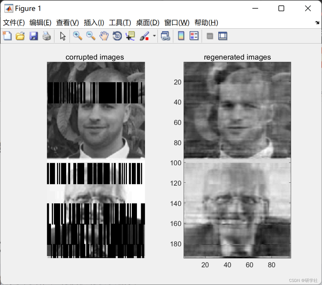
Part of the code:
pathname = uigetdir;allfiles = dir(fullfile(pathname,’*.jpg’));xts=[]; % initialize testing inputsfor i=1:size(allfiles,1) x=imread([pathname ‘\’ allfiles(i).name]);x=imresize(x,gamma);x=rgb2gray(x);x=double(x);xts=[xts; x];% testing set buildingend
%% Initialization of the AlgorithmNumberofHiddenNeurons=500; % number of neuronsD_ratio=0.35; % the ratio of noise in each chosen frameDB=1; % the power of white gaussian noise in decibels ActivationFunction=’sig’; % Activation functionframe=20; % size of each frame%% Train and test%%% % During training, gaussian white noise and zeros will be added to % randomly chosen frames .% The Autoencoder will be trained to avoid this type of data corruption.
[AE_net]=elm_AE(xtr,xts,NumberofHiddenNeurons,ActivationFunction,D_ratio,DB,frame)%% Important Note: %%% % After completing the training process, we will no longer need to use % InputWeight for mapping the inputs to the hidden layer, and instead of % that we will use the Outputweights beta for coding and decoding phases% and also we can’t use the activation function because beta is computed % after the activation .% The same thing is applied on biases (please for more details check the % function ‘ELM_AE’ at the testing phase).
%% Illustrationsubplot(121)corrupted=AE_net.x(:,1:gamma(2)*2);imshow(corrupted’)title(‘corrupted images ‘);subplot(122)regenerated=AE_net.Ytr_hat(:,1:gamma(2)*2);imagesc(regenerated’), colormap(‘gray’);title(‘regenerated images’);
%% scale training datasetT=Tinputs’;T = scaledata(T,0,1);% memorize original copy of the input and use it as a targetP=Tinputs’;%% scale training datasetTV.T=Tsinputs’;TV.T = scaledata(TV.T,0,1);% memorize original copy of the input and use it as a targetTV.P=Tsinputs’;TV.P = scaledata(TV.P,0,1);% temporal inputTVT=TV.T;%save a copy as an output of the function
%% in the 1st and 2nd step we will corrupt the temporal inputPtNoise=zeros(size(P));i=1;while i < size(P,2)-framegen=randi([0,1],1,1);PNoise=[];
%%% 1st step: generate set of indexes to set some input’s values to zero later %%% (here we set them randomly and you can choose them by probability)%%%[zeroind] = dividerand(size(P,1),1-D_ratio,0,D_ratio);% generate indexes%%% 2nd step: add gaussian noise if gen==1Noise=wgn(1,size(P,1),DB)’;% generate white gaussian noiseelseNoise=zeros(1,size(P,1))’; end
for j=1:frame;%copy noisePNoise=[PNoise Noise];endif gen==1for j=1:length(zeroind);% set to zero PNoise(zeroind(j),:)=0; P(zeroind(j),i:i+frame)=0;endend
PtNoise(:,i:i+frame-1)=PNoise;i=i+frame;end
🎉3 References
Some theoretical sources are from the internet. If there is any infringement, please contact for removal.
[1]P. Vincent, H. Larochelle, I. Lajoie, Y. Bengio, and P.-A. Manzagol, “Stacked Denoising Autoencoders: Learning Useful Representations in a Deep Network with a Local Denoising Criterion,” J. Mach. Learn. Res., vol. 11, no. 3, pp. 3371–3408, 2010. [2]L. le Cao, W. bing Huang, and F. chun Sun, “Building feature space of extreme learning machine with sparse denoising stacked-autoencoder,” Neurocomputing, vol. 174, pp. 60–71, 2016. [3]G. Bin Huang, “What are Extreme Learning Machines? Filling the Gap Between Frank Rosenblatt’s Dream and John von Neumann’s Puzzle,” Cognit. Comput., vol. 7, no. 3, pp. 263–278, 2015.