
The code implements a two-dimensional combined navigation system based on the Unscented Kalman Filter (UKF), integrating data from the Inertial Measurement Unit (IMU) and the Global Navigation Satellite System (GNSS). This system employs an 8-dimensional error state model to estimate the carrier’s position, velocity, attitude, and sensor biases in real-time.
Program Overview
System Overview
- IMU (Inertial Measurement Unit): Similar to the human inner ear, it senses acceleration and rotation.
- GNSS (Global Navigation Satellite System): Similar to GPS, it provides accurate location information.
Core Technology: Unscented Kalman Filter (UKF)
The traditional Extended Kalman Filter requires linearization of complex nonlinear equations, akin to approximating curves with straight lines, which introduces errors. The UKF employs a smarter approach:
- Accurate Sampling: Selecting key “sampling points” to represent the distribution of the entire system state.
- Direct Propagation: Allowing these sampling points to pass directly through the actual nonlinear equations.
- Statistical Reconstruction: Reconstructing the statistical characteristics of the system state from the propagated sampling points.
This is like having multiple scouts take different routes and then aggregating the information to find the best path, which is more accurate than simple linear approximations.
System State Design
8-Dimensional State Vector
The system tracks 8 key state variables:
Position Information (2D)
- X-direction position: The carrier’s coordinate in the east-west direction.
- Y-direction position: The carrier’s coordinate in the north-south direction.
Velocity Information (2D)
- X-direction velocity: The carrier’s speed in the east-west direction.
- Y-direction velocity: The carrier’s speed in the north-south direction.
Attitude Information (1D)
- Heading angle: The carrier’s orientation, equivalent to a compass reading.
Sensor Biases (3D)
- Gyroscope bias: Systematic error of the gyroscope.
- X-direction accelerometer bias: Systematic error of the X-axis accelerometer.
- Y-direction accelerometer bias: Systematic error of the Y-axis accelerometer.
Low-Frequency GNSS Data Fusion
GNSS provides accurate position information at a lower frequency (1Hz, once per second):
GNSS Data Characteristics:
- High accuracy: Typically achieves meter-level precision.
- Low frequency: Updates slowly, unable to capture rapid movements.
- Environmentally affected: May fail in tunnels or between tall buildings.
Fusion Strategy: When GNSS data is available, the system will:
- Compare GNSS observed position with IMU estimated position.
- Calculate the difference (innovation) between the two.
- Assign weights based on the reliability of each sensor.
- Intelligently correct the entire state estimate.
Algorithm Workflow
Prediction Phase
At each time step, the system predicts based on the current state and IMU data:
- Generate Sampling Points: Create multiple representative sampling points around the current state.
- State Propagation: Propagate each sampling point through the motion model to the next time step.
- Statistical Summary: Calculate the predicted state and uncertainty from the propagated sampling points.
Update Phase
When GNSS observation data is received:
- Observation Prediction: Predict the observation values corresponding to each sampling point.
- Calculate Gain: Compute the Kalman gain based on predicted uncertainty and observation noise.
- State Correction: Use the gain matrix to fuse observation information and correct the state estimate.
- Covariance Update: Update the uncertainty of the state estimate.
Simulation Validation Scenarios
Motion Model
The code simulates a typical test scenario: the carrier moves uniformly along a circular trajectory with a radius of 50 meters. This trajectory features:
- Continuous acceleration changes (centripetal acceleration).
- Constant angular velocity.
- Predictable true trajectory for performance evaluation.
Sensor Simulation
IMU Sensor Simulation:
- Add random noise to the actual acceleration and angular velocity.
- Simulate the random walk characteristics of sensor biases.
- Consider the noise levels of actual sensors.
GNSS Sensor Simulation:
- Add Gaussian white noise to the actual position.
- Simulate a lower update frequency.
- Intermittently provide observation data.
Performance Evaluation and Comparison
Comparison Benchmarks
The code provides a comparison of three navigation schemes:
Pure IMU Integration:
- Advantages: High frequency, high short-term accuracy, does not rely on external signals.
- Disadvantages: Severe error accumulation, noticeable long-term drift.
Pure GNSS Positioning:
- Advantages: No accumulated errors, long-term stability.
- Disadvantages: Low update frequency, poor dynamic response, signals easily interrupted.
UKF Combined Navigation:
- Combines the advantages of both: high frequency + long-term stability.
- Intelligent error correction: Automatically calibrates sensor biases.
- Strong robustness: Can still operate when a single sensor fails.
Performance Metrics
The system uses Root Mean Square Error (RMSE) to evaluate performance:
- Position RMSE: Reflects positioning accuracy.
- Velocity RMSE: Reflects velocity estimation accuracy.
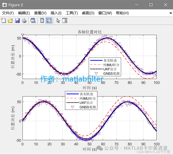
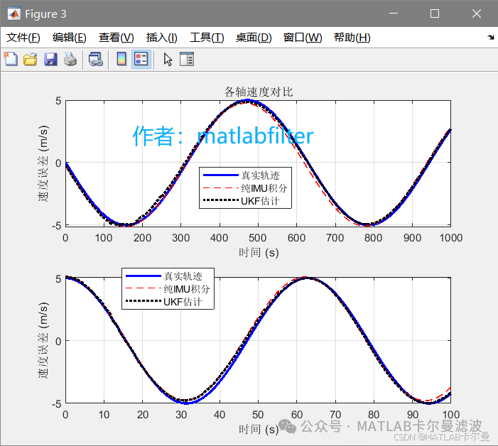
<span>Typical results show that the accuracy of UKF combined navigation significantly outperforms single sensor schemes.</span>
Running Results
2D trajectory image comparison: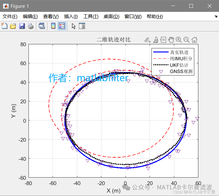 Comparison of position curves in two dimensions:
 Comparison of velocity curves in two dimensions:
 Error curve: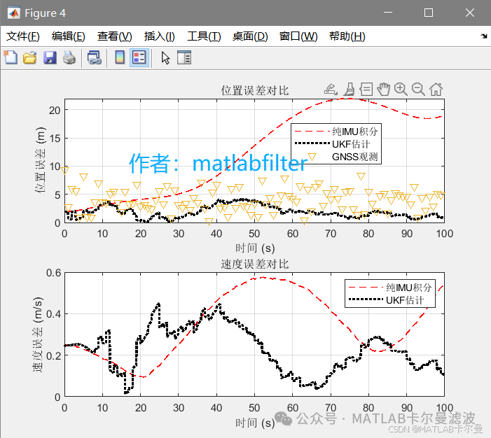
MATLAB Source Code
Part of the code is as follows:
% UKF routine for 2D state variables (with strict combined navigation derivation)
% Based on an 8-dimensional error state model: position, velocity, heading, gyroscope bias, accelerometer bias
% 4-dimensional observations: XY position (2)
% Author contact: WeChat matlabfilter (for paid consultations, unless previously agreed)
% 2025-08-28/Ver1

clear; clc; close all;
rng(0);% Fix random seed

%% System parameter settings
dt =0.1;% Sampling time interval (s)
total_time =100;% Total simulation time (s)
N = total_time / dt;% Number of sampling points

%% Noise parameter settings
% IMU noise parameters
gyro_noise_std =0.1*pi/180;% Gyroscope noise standard deviation (rad/s)
accel_noise_std =0.01;% Accelerometer noise standard deviation (m/s^2)
gyro_bias_std =0.01*pi/180;% Gyroscope bias standard deviation (rad/s)
accel_bias_std =0.001;% Accelerometer bias standard deviation (m/s^2)

% GNSS observation noise
gnss_pos_noise_std =3;% GNSS position noise standard deviation (m)

%% Process noise covariance matrix Q (8×8)
% State order: [position(2), velocity(2), attitude(1), gyroscope bias(1), accelerometer bias(2)]
Q =zeros(8,8);
% Position noise (generated by velocity integration)
Q(1:2,1:2)=eye(2)*(accel_noise_std * dt^2)^2;
% Velocity noise
Q(3:4,3:4)=eye(2)*(accel_noise_std * dt)^2;
% Attitude noise
Q(5,5)=eye(1)*(gyro_noise_std * dt)^2;
% Gyroscope bias noise
Q(6,6)=eye(1)*(gyro_bias_std * dt)^2;
% Accelerometer bias noise
Q(7:8,7:8)=eye(2)*(accel_bias_std * dt)^2;

%% Observation noise covariance matrix R (2×2)
% Observations: GNSS position(2)
R =eye(2)* gnss_pos_noise_std^2;

%% Initialization
% True trajectory parameters (circular motion)
radius =50;% Circular trajectory radius (m)
Complete code download link:
https://mall.bilibili.com/neul-next/detailuniversal/detail.html?isMerchant=1&page=detailuniversal_detail&saleType=10&itemsId=13019758&loadingShow=1&noTitleBar=1&msource=merchant_share
Or click “Read the original text” at the end to jump.
<span>If you need assistance or have custom code requirements related to navigation and positioning filtering, please contact the author via WeChat below.</span>