Reading, Interpolating, and Plotting ERA5 Data in MATLAB

Click the blue text

Follow us

1

Reading nc files in MATLAB

After downloading the ERA5 data (for download instructions, refer to the ERA5 data CDS API download (Windows system)), the data format is .nc files. Therefore, it is necessary to read, understand the nc files, and plot the distribution of relevant variables.

• View nc file——ncdisp

Example: ncdisp(‘E:\ERA5\monthly\mon_tem_19402022.nc’)

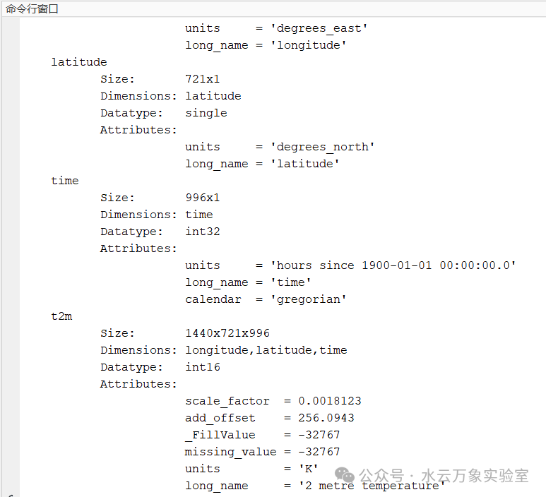
The main information of the nc file will be displayed in the command window: longitude, latitude, time, variables, etc.

• Read nc file——the MATLAB command is: ncread

  Example: ncread(‘E:\ERA5\monthly\mon_tem_19402022.nc’,‘t2m’);

2

Reading temperature data and interpolating in MATLAB

% Read data
pr=[];
tem=[];
% Start year and end year
st_year=1950;
ed_year=2014;
% ncdisp('E:\ERA5\monthly\mon_tem_19402022.nc')
tt=ncread('E:\ERA5\monthly\mon_tem_19402022.nc','t2m');

% Read longitude and latitude, and plot the original data image
lon=ncread('E:\ERA5\monthly\mon_tem_19402022.nc','longitude');
lat=ncread('E:\ERA5\monthly\mon_tem_19402022.nc','latitude');
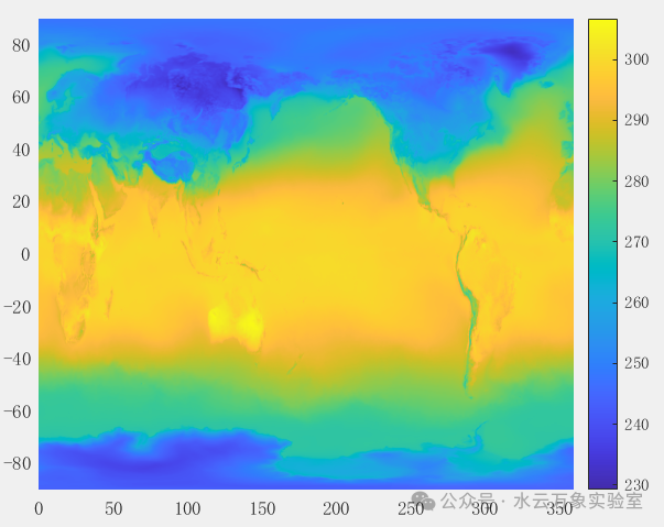
pcolor(lon,lat,tt(:,:,1)');
shading flat

The directly plotted original image looks like this (the African continent is separated).

However, the world map base we generally use for scientific plotting is in this form.

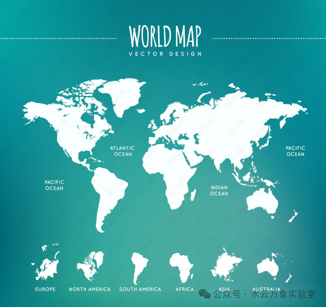
Therefore, we need to flip the original ERA5 data left and right:

% Flip the map (left-right flip)
[m,n,k]=size(tt);
dt1=zeros(m,n,k);
dt1(1:length(tt)/2,:,:)=tt(length(tt)/2+1:end,:,:);
dt1(length(tt)/2+1:end,:,:)=tt(1:length(tt)/2,:,:);

The flipped data dt1 is then plotted again:

pcolor(lon,lat,dt1(:,:,1)');
shading flat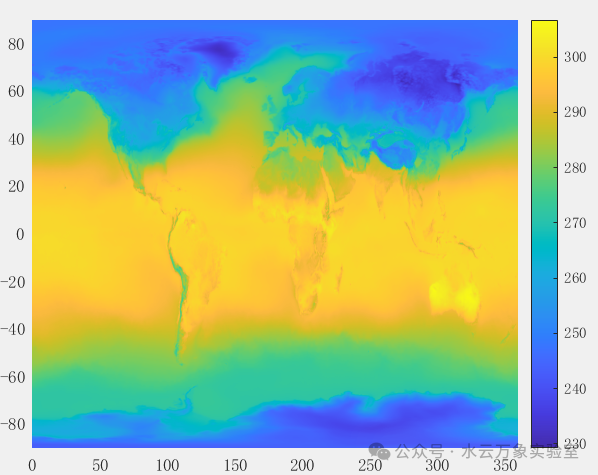

You can see that the image has been corrected.

Next, we perform interpolation (MATLAB function: interp2), which means interpolating the data to the desired resolution. The original ERA5 resolution is 0.25, and here we interpolate to 2. (tem is the data after interpolation).

%% Interpolating ERA5 data
% Interpolating to 2*2
x=lon';
y=lat;
x0=repmat(x,length(y),1);
y0=repmat(y,1,length(x));
h=2;    % Interpolation longitude and latitude
nlon=0:h:359.75;
nlat=89.75:-h:-89.75;
[xi,yi] = meshgrid(nlon,nlat);
for j=1:k
    nd=dt1(:,:,j)';
    tem(:,:,j)=interp2(x0,y0,nd,xi,yi,'nearest')';
end

2

Plotting temperature images in MATLAB

Note:

% The longitude and latitude before flipping are: lon:0~359.75; lat:-90~90

% The longitude and latitude after flipping are: lon:-180~179.75; lat:-90~90

% When plotting, use the longitude and latitude corresponding to the flipped data

h=2;    % Plotting longitude and latitude
nlon=-180:h:179.75;
nlat=89.75:-h:-89.75;
pcolor(nlon,nlat,dt(:,:,1)');
shading flat
hold on;
land = shaperead('landareas.shp');
plot(extractfield(land,'X'),extractfield(land,'Y'),'k','LineWidth',1);
colorbar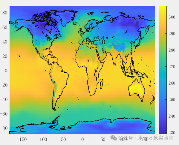

If you need the complete code, please message us privately for a free share.

* Please do not directly copy content from this public account; please indicate the source when reprinting *