Kriging

1. Kriging Response Surface

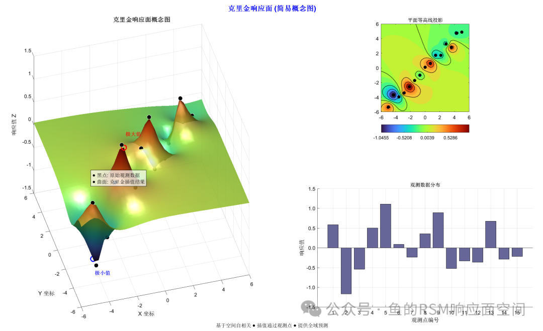
Kriging is a spatial correlation-based interpolation and prediction method.

It effectively constructs the mapping relationship between input variables and output responses.

Core Idea

The response is viewed as a combination of global trends and local spatial deviations:

全局趋势局部波动

• • Global Trend ()： Described by regression models.
• • Local Spatial Deviation ()： Characterized by a zero-mean, spatially correlated stationary random process, capturing local fluctuations not explained by the regression model.

2. Mathematical Principles

1. Prediction (Kriging Predictor)

Given a set of n dimensional design points and their corresponding m responses

The predicted value at the unknown point x is:

全局趋势局部波动

• • : Global trend approximation
• • : Regression basis functions (also known as basis function vector).
• • : Generalized least squares estimate of regression coefficients ( matrix).
• • : Local spatial correction
• • : The correlation vector between point x and all design points (), directly calculated from the correlation function.
• • : Spatial correction weights ( matrix), obtained by solving the residual equation (where is the correlation matrix between design points).
• • Combination Meaning: Predicted value = Global trend estimate + Weighted correction of residuals based on spatial correlation.

2. Regression Models

Regression models play the role of global trend modeling. Its general form is:

where represents the response component.

• • : Regression model for the th response component
• • : Regression coefficient of the th basis function ().
• • : The th basis function
• • : Basis function vector
• • : Regression coefficient vector

The DACE toolbox provides three commonly used polynomial regression models:

3. Spatial Correlation (Correlation Models)

The key characteristics of local spatial deviation are defined by its covariance function:

• • : Process variance (Process Variance) scaling factor, controlling the overall fluctuation amplitude without affecting the spatial correlation pattern.
• • : Correlation function (Correlation Function) core lies in defining the strength of correlation between any two points and . Typically, a product form of anisotropy is used: .
• • Parameter controls the rate of decay of correlation with distance in different directions (). Optimized through maximum likelihood estimation, with the objective function being .

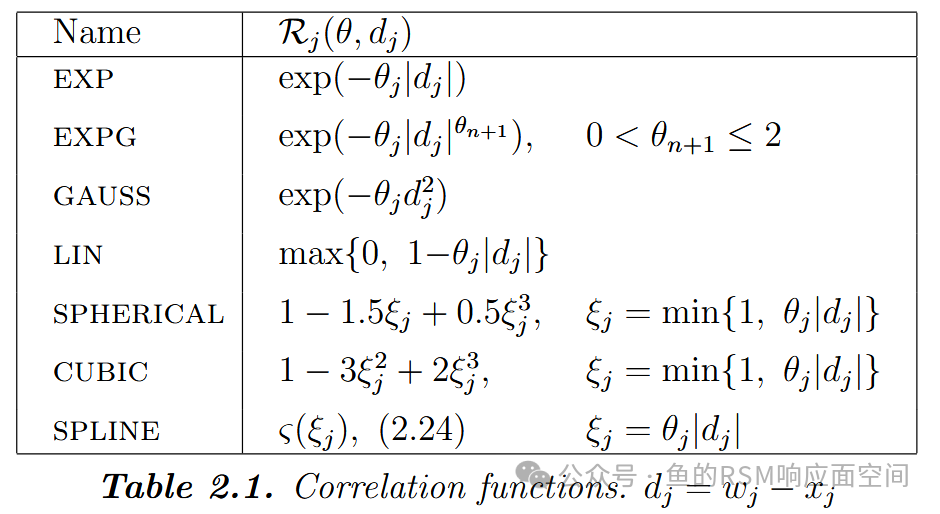
The DACE toolbox provides various correlation functions (behavior controlled by ):

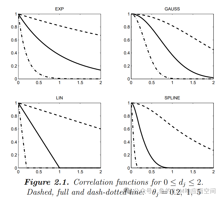
Legend: Variation of correlation functions with distance under different (0.2, 1, 5). Dashed line (), solid line (), dotted line ().

3. Unique Advantages of Kriging Model

1. 1. Accurate Interpolation: Predicted values at known design points are strictly equal to observed values ().
2. 2. Built-in Error Estimation (MSE): Provides mean squared error estimates at prediction points . This error increases in areas far from design points and is zero at known design points.
3. 3. Flexible Modeling: Both regression models and correlation functions can be flexibly selected and customized based on problem characteristics.

It can be seen that the construction process of the Kriging model mainly involves: selection of sample points, regression models, and correlation functions.

4. MATLAB-DACE Toolbox

Core Workflow (Function Syntax)

1. 1. Model Construction (<span>dacefit</span>)：

   [dmodel, perf] = dacefit(S, Y, @regr_func, @corr_func, theta0, lob, upb);

• • <span>@regr_func</span>: Regression function handle (e.g., @regpoly0, @regpoly1, @regpoly2, custom function).
• • <span>@corr_func</span>: Correlation function handle (e.g., @corrgauss, @correxp, @corrspline, custom function).
• • <span>theta0</span>: Initial or fixed value of correlation parameters .
• • <span>lob</span>, <span>upb</span> (optional): Lower and upper bounds for . If provided, optimization will occur; if not, <span>theta0</span> will be used as a fixed value.
• • dmodel: Returned model structure (including , scaling factors, etc.).
• • perf: Optimization process information (number of evaluations, parameter trajectory).

[y_pred, dy_pred, mse, dmse] = predictor(X, dmodel);

• • <span>X</span>: Matrix containing n prediction points.
• • <span>y_pred</span>: Predicted response.
• • <span>dy_pred</span> (optional): Jacobian (gradient) of predicted response with respect to inputs.
• • <span>mse</span> (optional): Mean squared error (MSE) of predictions.
• • <span>dmse</span> (optional): Jacobian (gradient) of MSE with respect to inputs.

Example: Response Surface Fitting

% 1. Load data (document example, see the same path as the toolbox download)
load data1.mat;  % Contains 75x2 design points S, 75x1 response Y (region [0,100]^2)

% 2. Set model options
regr = @regpoly0;        % Constant regression (zero-order polynomial)
corr = @corrgauss;       % Gaussian correlation function
theta0 = [10; 10];      % Initial theta (isotropic assumption starting point)
lob = [0.1; 0.1];       % Lower bound for theta
upb = [20; 20];         % Upper bound for theta (triggers optimization)

% 3. Fit Kriging model
dmodel, perf] = dacefit(S, Y, regr, corr, theta0, lob, upb);

% 4. Generate 40x40 prediction grid in the region [0,100]x[0,100]
X = gridsamp([0 0; 100 100], 40);

% 5. Predict response and MSE at grid points
[YX, MSE] = predictor(X, dmodel);   % Get predicted values YX and mean squared error MSE

% 6. Visualize prediction surface and design points
X1 = reshape(X(:, 1), 40, 40);     % Grid X1 coordinates
X2 = reshape(X(:, 2), 40, 40);     % Grid X2 coordinates
YX_grid = reshape(YX, 40, 40);     % Reshape predicted values to grid

figure(1);
mesh(X1, X2, YX_grid);             % Plot prediction surface
xlabel('x1'); ylabel('x2'); zlabel('Predicted y');
hold on;
plot3(S(:, 1), S(:, 2), Y, '.k', 'MarkerSize', 10); % Overlay original design points
hold off;
title('Kriging Prediction Surface');

% 7. (Optional) Visualize mean squared error surface
figure(2);
mesh(X1, X2, reshape(MSE, 40, 40));
xlabel('x1'); ylabel('x2'); zlabel('MSE');
title('Mean Squared Error (MSE)');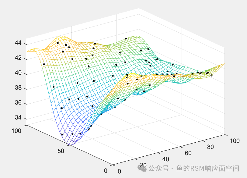

Legend: Kriging prediction surface based on constant regression and Gaussian correlation, with black points representing original design points.

5. Application Scenarios

1. 1. Surrogate Models for Computer Experiments: Substitute for expensive simulation programs (e.g., CFD) for rapid exploration of design space, parameter studies, and visualization.
2. 2. Proxy Models: Develop efficient sequential sampling strategies by combining predicted values and MSE to guide new experimental point placements.
3. 3. Spatial Data Interpolation: Interpolation and mapping of spatially distributed data in fields such as geostatistics and environmental monitoring.

Difference (Kriging vs. RSM):

• • Kriging:

Explicitly models the spatial correlation of data, achieving higher fitting accuracy for deterministic simulation data, especially suitable for nonlinear systems.

• • Traditional RSM (Polynomial Regression):

Only uses regression models to fit global trends, ignoring spatial correlation. Accuracy may be insufficient in cases of strong nonlinearity or significant local features.

DACE Toolbox Download Process:1. Download the DACE toolbox from the following website

https://www.omicron.dk/dace.html

2. Download to the toolbox folder under the MATLAB path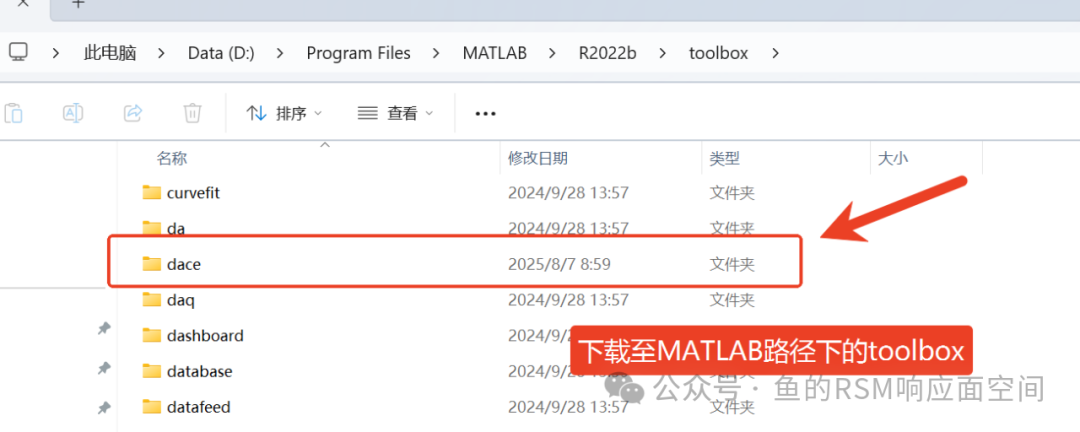3. Specify the toolbox path in the MATLAB command line and check if the toolbox is successfully installed

% Temporarily add toolbox path (specify the actual path where DACE is downloaded, only valid for current session)
addpath('D:\Program Files\MATLAB\R2022b\toolbox\dace');% Permanently save path (to include this path in all future sessions)
savepath;
% Check if core functions exist
which predictor
which regpoly0
if exist('dacefit', 'file') == 2  
disp('DACE toolbox installed');
else  
disp('DACE toolbox not found');
end

4. Note: Help documentation and official examples are in the DACE folder