Introduction
During the process of model evaluation, it is often necessary to assess the simulation performance of the model, which is typically represented by the correlation coefficient (CC), relative standard deviation (SD), and the centered root mean square error (RMSE). These three metrics can often be specifically illustrated using a Taylor diagram. The closer the RMSE is to 0, and the closer CC and SD are to 1, the better the model’s simulation capability.
1. Data Preprocessing
Meteorological grid data is usually three-dimensional, but when calculating CC, SD, and RMSE, it is often necessary to convert it into a one-dimensional array for computation. Therefore, preprocessing of the meteorological grid data is required.
import geopandas as gpd
import salem
# Create mask data
shp = "E:/shapefile/青藏高原/青藏高原边界数据总集/TPBoundary_HF/TPBoundary_HF_LP.shp"
tp_shp=gpd.read_file(shp)
data0=xr.open_dataset('E:/CORDEX-DOMAIN/conclusion/pr/RX1day.nc')
RX1day=data0.RX1day
data1=xr.open_dataset('E:/CORDEX-DOMAIN/conclusion/pr/RX1day1.nc')
RX1day1=data1.RX1day
data2=xr.open_dataset('E:/CORDEX-DOMAIN/conclusion/pr/RX1day2.nc')
RX1day2=data2.RX1day
data3=xr.open_dataset('E:/CORDEX-DOMAIN/conclusion/pr/RX1day3.nc')
RX1day3=data3.RX1day
RX1day=RX1day.salem.roi(shape=tp_shp)
RX1day1=RX1day1.salem.roi(shape=tp_shp)
RX1day2=RX1day2.salem.roi(shape=tp_shp)
RX1day3=RX1day3.salem.roi(shape=tp_shp)
# Reduce three-dimensional array to one-dimensional
# [Data Reorganization and Reshaping](https://www.jianshu.com/p/3e2eecd6481d)
RX1day=RX1day.stack(z=('time', 'lat','lon'))
RX1day1=RX1day1.stack(z=('time', 'lat','lon'))
RX1day2=RX1day2.stack(z=('time', 'lat','lon'))
RX1day3=RX1day3.stack(z=('time', 'lat','lon'))
DATA={"RX1day": RX1day,  "RX1day1": RX1day1,  "RX1day2": RX1day2,  "RX1day3": RX1day3,  }
df = pd.DataFrame(DATA)
df1=df.dropna(axis=0,subset = ["RX1day","RX1day1","RX1day2","RX1day3"])   # Discard rows with missing values in these four columns
2. Steps to Use
1. Import Libraries
The code is as follows (example):
from matplotlib.projections import PolarAxes
from mpl_toolkits.axisartist import floating_axes
from mpl_toolkits.axisartist import grid_finder
import numpy as np
import matplotlib.pyplot as plt
2. Read Data
The code is as follows (example):
def set_tayloraxes(fig, location):
    trans = PolarAxes.PolarTransform()
    r1_locs = np.hstack((np.arange(1,10)/10.0,[0.95,0.99]))
    t1_locs = np.arccos(r1_locs)
    gl1 = grid_finder.FixedLocator(t1_locs)
    tf1 = grid_finder.DictFormatter(dict(zip(t1_locs, map(str,r1_locs))))
    r2_locs = np.arange(0,2,0.25)
    r2_labels = ['0 ', '0.25 ', '0.50 ', '0.75 ', 'REF ', '1.25 ', '1.50 ', '1.75 ']
    gl2 = grid_finder.FixedLocator(r2_locs)
    tf2 = grid_finder.DictFormatter(dict(zip(r2_locs, map(str,r2_labels))))
    ghelper = floating_axes.GridHelperCurveLinear(trans,extremes=(0,np.pi/2,0,1.75),
                                                  grid_locator1=gl1,tick_formatter1=tf1,
                                                  grid_locator2=gl2,tick_formatter2=tf2)
    ax = floating_axes.FloatingSubplot(fig, location, grid_helper=ghelper)
    fig.add_subplot(ax)
    ax.axis["top"].set_axis_direction("bottom")
    ax.axis["top"].toggle(ticklabels=True, label=True)
    ax.axis["top"].major_ticklabels.set_axis_direction("top")
    ax.axis["top"].label.set_axis_direction("top")
    ax.axis["top"].label.set_text("Correlation")
    ax.axis["top"].label.set_fontsize(14)
    ax.axis["left"].set_axis_direction("bottom")
    ax.axis["left"].label.set_text("Standard deviation")
    ax.axis["left"].label.set_fontsize(14)
    ax.axis["right"].set_axis_direction("top")
    ax.axis["right"].toggle(ticklabels=True)
    ax.axis["right"].major_ticklabels.set_axis_direction("left")
    ax.axis["bottom"].set_visible(False)
    ax.grid(True)
    polar_ax = ax.get_aux_axes(trans)
    rs,ts = np.meshgrid(np.linspace(0,1.75,100),
                        np.linspace(0,np.pi/2,100))
    rms = np.sqrt(1 + rs**2 - 2*rs*np.cos(ts))
    CS = polar_ax.contour(ts, rs,rms,colors='gray',linestyles='--')
    plt.clabel(CS, inline=1, fontsize=10)
    t = np.linspace(0,np.pi/2)
    r = np.zeros_like(t) + 1
    polar_ax.plot(t,r,'k--')
    polar_ax.text(np.pi/2+0.032,1.02, " 1.00", size=10.3,ha="right", va="top",
                  bbox=dict(boxstyle="square",ec='w',fc='w'))
    return polar_ax

def plot_taylor(axes, refsample, sample, *args, **kwargs):
    std = np.std(refsample)/np.std(sample)
    corr = np.corrcoef(refsample, sample)
    theta = np.arccos(corr[0,1])
    t,r = theta,std
    d = axes.plot(t,r, *args, **kwargs)
    return d
Usage of the two functions:
(1) set_tayloraxes(fig, location)
Input:
fig: The figure to be plotted
location: The position of the plot, e.g., 111 for the first in a 1×1 grid, 122 for the second in a 1×2 grid
Output:
polar_ax: Taylor coordinate system
(2) plot_taylor(axes, refsample, sample, *args, **kwargs)
Input:
axes: The Taylor coordinate system returned by setup_axes
refsample: Reference sample
sample: Evaluation sample
args, *kwargs: Relevant parameters for the plt.plot() function, to set point colors, shapes, etc.
fig = plt.figure(figsize=(12,6))
ax1 = set_tayloraxes(fig, 121)
d1 = plot_taylor(ax1,df1.RX1day,df1.RX1day1, 'ro',markersize=8,label='RX1day')
d2 = plot_taylor(ax1,df1.RX1day,df1.RX1day2, 'yo',markersize=8,label='TXn')
d3 = plot_taylor(ax1,df1.RX1day,df1.RX1day3, 'mo',markersize=8,label='TX90p')
d4 = plot_taylor(ax1,df1.RX1day,df1.RX1day, 'go',markersize=8,label='TX10p')
ax1.legend(loc=2)
ax2 = set_tayloraxes(fig, 122)
d1 = plot_taylor(ax2,df1.RX1day,df1.RX1day1, 'ro',markersize=8,label='RX1day')
d2 = plot_taylor(ax2,df1.RX1day,df1.RX1day2, 'yo',markersize=8,label='TXn')
d3 = plot_taylor(ax2,df1.RX1day,df1.RX1day3, 'mo',markersize=8,label='TX90p')
d4 = plot_taylor(ax2,df1.RX1day,df1.RX1day, 'go',markersize=8,label='TX10p')
# Legend position
ax2.legend(bbox_to_anchor=(1.32,0.8), borderaxespad=0)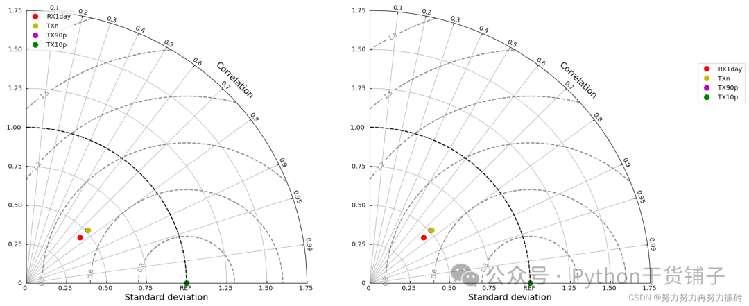
————————————————
Copyright Statement: This article is an original work by CSDN blogger “努力努力再努力搬砖”. Please include the original source link and this statement when reprinting.
Original link: https://blog.csdn.net/weixin_43347581/article/details/129682668