Original link: https://tecdat.cn/?p=35748

Video source: Tuoduan Douyin account @Tuoduan tecdat

Copula is a function used to describe the correlation between multiple random variables, connecting their joint distribution with their marginal distributions. The copula function is defined by Sklar’s theorem, which states that for the joint distribution of N random variables, it can be decomposed into the marginal distributions of these N variables and a copula function. (Click “Read the original” at the end to obtain the complete code data)

Related videos

In this way, the randomness and coupling of the variables are separated, where the randomness of each random variable is described by the marginal distribution, while the coupling characteristics between random variables are described by the copula function.

This article aims to demonstrate how to use copulas in Python for multivariate joint distribution modeling and visualization through a series of examples. We will start with a simple bivariate copula model and gradually transition to more complex multivariate models, introducing how to use different types of copulas and parameters to fit different data characteristics.

1. Copulas in Multivariate Joint Distribution Modeling

Copula functions have wide applications in fields such as financial risk management, actuarial science, and statistical inference. They encompass all dependency information of random variables, making them very useful for analyzing the relationships between variables, especially when traditional linear correlation coefficients may not accurately measure the relationships.

Specifically, a copula function is a mapping from [0,1]^n to [0,1], used to link the marginal cumulative distribution functions of n random variables. It describes the dependency relationships between multivariate random variables, which can be positively correlated, negatively correlated, or uncorrelated.

When modeling systems, it is common to encounter situations involving multiple parameters. Each of these parameters can be described by a given probability density function (PDF). If we want to generate a set of new parameter values, we need to sample from these distributions (also known as marginal distributions). There are mainly two cases: (i) the PDFs are independent; (ii) there is a dependency relationship. One way to model the dependency relationship is to use copulas.

Kaizong Ye

Tuoduan Analyst

Sampling from Copulas

Let us illustrate with a bivariate example, assuming we have prior knowledge and know how to model the dependency relationship between two variables.

In this case, we use the Gumbel copula and fix its hyperparameter theta=2. We can visualize its two-dimensional PDF.

_ = copulot_pdf()  # Visualization

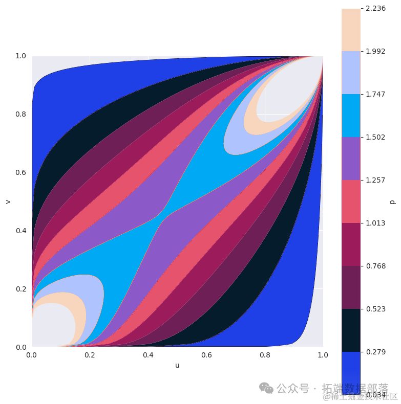
And we can sample from this PDF.

rng = np.random.default_rng(seed)

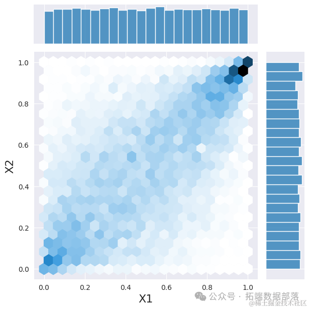
Now let us return to these two variables. In this case, we consider them to follow a gamma distribution and a normal distribution. If they are independent of each other, we can sample from each PDF separately. Here we use a convenient class to perform the same operation.

Click the title to check previous content

R language multivariate Copula GARCH model time series prediction

Swipe left to see more

01

02

03

04

Reproducibility

Generating reproducible random values from copulas requires explicitly setting the seed parameter. The seed accepts an initialized NumPy Generator or RandomState, or any parameter that np.random.default_rng can accept, such as an integer or a tuple of integers. In this example, an integer is used.

Direct exposure to the singleton RandomState in np.random distributions will not be used, and setting np.random.seed has no effect on the generated values.

_ = h.set_labels("X1", "X2", fontsize=16)

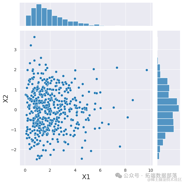
Now that we have expressed the dependency relationship between the variables using copulas, we can use the same convenient class to sample a new set of observations from this copula.

	# Using an initialized Generator object  

	h = snjoind="scatter")

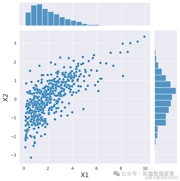
There are two points to note. (i) Just like in the independent case, the marginal distributions correctly display the gamma and normal distributions; (ii) The dependency relationship between the two variables is visible.

Estimating Copula Parameters

Now, suppose we have experimental data and know that we can use the Gumbel copula to express the dependency relationship. However, we do not know the values of the copula’s hyperparameters. In this case, we can estimate this value.

We will use the samples generated earlier, as we already know the hyperparameter value we should obtain: theta=2.

fit_carm(sample)
print(theta)

We can see that the estimated hyperparameter value is close to the previously set value.

2. Copulas in Python: Estimation and Visualization of Frank, Clayton, and Gumbel Copula Models

Most of the content that will appear in this article will be built using Jupyter Notebooks.

Software

There is no explicit implementation of copula packages in scikit-learn or scipy.

Frank, Clayton, and Gumbel Copulas for 2D Data

Testing

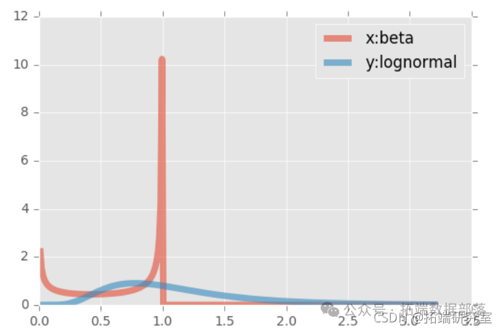
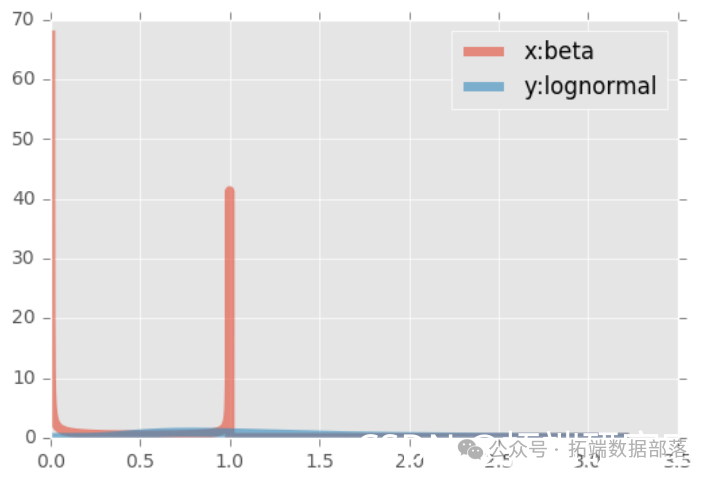
The first sample (x) is generated from a beta distribution, and (y) is generated from a log-normal distribution. The support of the beta distribution is limited, while the right support of the log-normal distribution is infinite. One interesting property of the logarithm. Both marginals are transformed to the unit range.

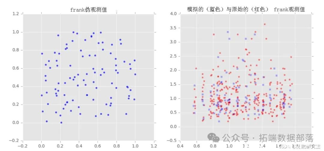
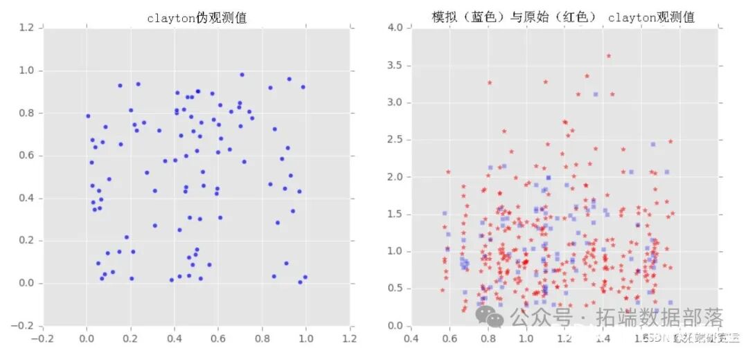
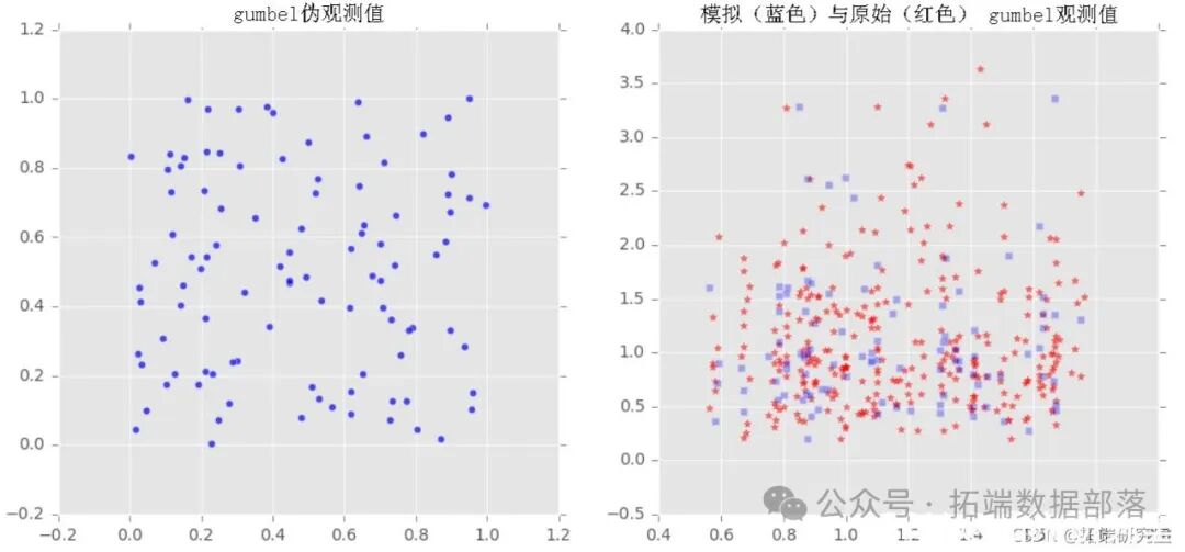
We fitted copulas from three families (Frank, Clayton, Gumbel) to samples x and y, then extracted some samples from the fitted copulas and plotted the sampling output alongside the original samples to observe their comparison.

    # Equivalent to ppf, but built directly from data 
    sortedvar=np.sort(var)    

    # Plotting

    for index,family in enumerate(['Frank', 'clayton', 'gumbel']):

            # Obtain pseudo-observations
            u,v = copula_f.generate_uv(howmany)

        # Plot pseudo-observations
        axs[index][0].scatter(u,v,marker='o',alpha=0.7)


    plt.show()

# Comparison of total samples and pseudo-observations
sz=300
loc=0.0 # Required for most distributions
sc=0.5
y=lognorm.rvs(sc,loc=loc, size=sz)

Independent (Uncorrelated) Data

We will draw samples (x) from the beta distribution and (y) from the log-normal distribution. These samples are pseudo-independent (we know that if you sample with a computer, there will not be true independence, but it is reasonably independent).

# Uncorrelated data: a beta (x) and a log-normal (y).
a= 0.45#2. #alpha
b=0.25#5. #beta

# Plot uncorrelated x and y 
plt.plot(t, beta.pdf(t,a,b), lw=5, alpha=0.6, label='x:beta')


# Plot the copula established by uncorrelated x and y 
title='Copula from uncorrelated data x: beta, alpha {} beta {}, y: lognormal, mu {}, sigma dPlot(title,x,y,pseudoobs)

Dependent (Correlated) Data

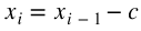
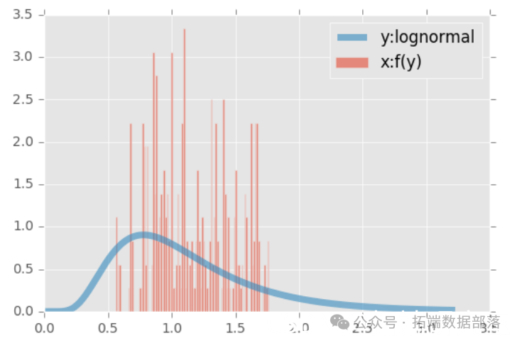
The independent variable will be a log-normal (y), and the variable (x) depends on (y), with the following relationship. The initial value is 1 (independent). Then, for each point i, if , then , where c is uniformly chosen from a list of fractions from 1; otherwise, .

# Correlated data: a log-normal (y).

# Plot correlated data

 np.linspace(0, lognorm.ppf(0.99, sc), sz)
plt.plot(t, gkxx.pdf(t), lw=5, alpha=0.6,

Fitting Copula Parameters

There is no built-in method to compute parameters for Archimedean copulas, nor for elliptical copulas. However, you can implement it yourself. Choose to fit some parameters to a scipy distribution, then use the CDF method of that function on some samples, or work with an empirical CDF. Both methods are implemented in the notebook.

Therefore, you have to write code yourself to obtain parameters for Archimedean copulas, transform the variables to a uniform marginal distribution, and perform actual operations on the copula. It is quite flexible.

# Method for fitting copula parameters 

# === Frank parameter fitting
    """
    Optimizing this function will yield parameters 
    """
   # Integral value of the first-order debye function    int_debye = lambda t: t/(npexp(t)-1.) 
    debye = lambda alphaquad(int_debye , 
                               alpha
                              )[0]/alpha
    diff = (1.-kTau)/4.0-(debye(-alpha)-1.)/alpha


#================
# Clayton parameter method
def Clayton(kTau):
    try:
        return 2.*kTau/(1.-kTau)


# Gumbel parameter method
def Gumbel(kTau):
    try:
        return 1./(1.-kTau)


#================
# Copula generation

    # Obtain covariance matrix P
    #x1=norm.ppf(x,loc=0,scale=1)
    #y1=norm.ppf(y,loc=0,scale=1)
    #return norm.cdf((x1,y1),loc=0,scale=P)


#================
# Copula plotting

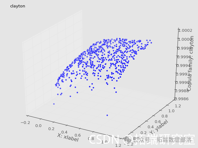
    fig = pylab.figure()
    ax = Axes3D(fig)

        ax.text2D(0.05, 0.95, label, transform=ax.transAxes)
        ax.set_xlabel('X: {}'.format(xlabel))
        ax.set_ylabel('Y: {}'.format(ylabel))


    # Sample is an index list from U,V. This way, we will not plot the entire copula curve.
    if plot:

        print "Plotting samples of copula {}".format(copulaName)
        returnable[copulaName]=copulapoints
        if plot:
            zeFigure=plot3d(U[样本],V[样本],copulapoints[样本], label=copulaName,

Generating Some Input Data

In this example, we use the same distributions as before to explore copulas. If you want to adapt this code to your own real data,.

t = np.linspace(0, lognorm.ppf(0.99, sc), sz)

# Sample some values from some df
X=beta.rvs(a,b,size=sz)
Y=lognorm.rvs(sc,size=sz)
# Implement marginal distributions by applying CDF to the values in the samples
U=beta.cdf(X,a,b)
V=lognorm.cdf(Y,sc)

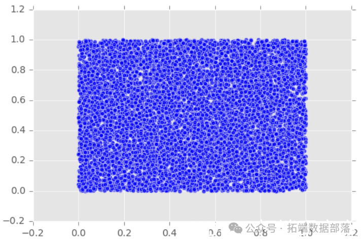
# Plot them to visually check independence
plt.scatter(U,V,marker='o',alpha=0.7)
plt.show()

Visualizing Copulas

There is no direct constructor for Gaussian or t Copulas, but a more general function can be established for elliptical Copulas (Elliptic Copulas).

Samples=700
# Choose copula index for sampling
np.random.choice(range(len(U)),Samples)

Plot(U,V)

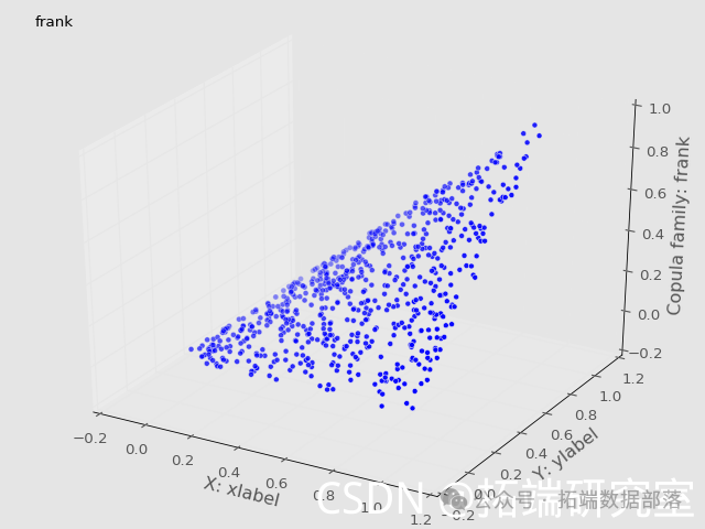
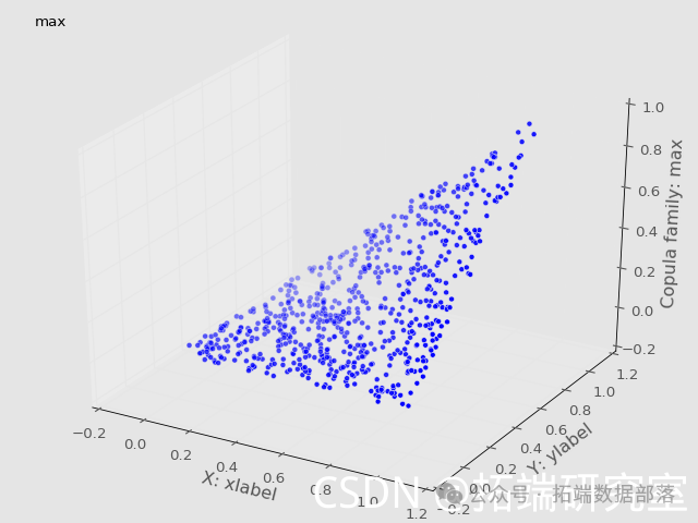
<IPython.core.display.Javascript object>

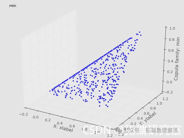
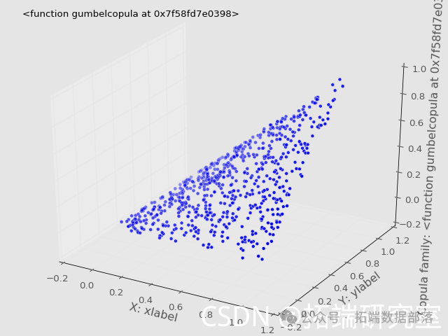
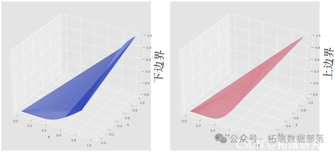
Visualization of Frechét-Höffding Boundaries

According to the theorem, we plot the copula together to obtain the Frechét-Höffding boundaries.

# Establish boundaries as regions of copulas
plot_trisurf(U[样本],V[样本],copula['min'][样本],
          c='red') # Upper limit
plot_trisurf(U[样本],V[样本],copula['max'][样本],
           c='green') # Lower limit

The data and code analyzed in this article are shared in the member group, scan the QR code below to join the group!

Click “Read the original” at the end to obtain the complete code data materials

This article is selected from “Visualization of Copulas in Multivariate Joint Distribution Modeling with Python: A Collection of 2 Examples”.

Click the title to check previous content

MATLAB simulation optimization of market risk data VaR analysis using CopulaR language ARMA GARCH COPULA model fitting stock return time series and simulation visualizationARMA-GARCH-COPULA model and financial time series caseTime series analysis: ARIMA GARCH model analysis of stock price dataGJR-GARCH and GARCH volatility prediction of the P/E index time series and Mincer Zarnowitz regression, DM test, JB test[Video] Time series analysis: ARIMA-ARCH / GARCH model analysis of stock pricesTime series GARCH model analysis of stock market volatilityPYTHON using GARCH, discrete stochastic volatility model DSV to simulate estimate stock return time series and Monte Carlo visualizationExtreme value theory EVT, POT threshold exceedance, GARCH model analysis of stock index VaR, conditional CVaR: diversified portfolio risk measure analysisGARCH volatility prediction regime-switching trading strategyFinancial time series model ARIMA and GARCH in stock market prediction applicationsTime series analysis model: ARIMA-ARCH / GARCH model analysis of stock pricesR language risk value: ARIMA, GARCH, Delta-normal method rolling estimate VaR (Value at Risk) and backtesting analysis of stock dataR language GARCH modeling commonly used software package comparison, fitting S&P 500 index volatility time series and prediction visualizationPython financial time series model ARIMA and GARCH in stock market prediction applicationsMATLAB fitting and predicting stock market return time series volatility using GARCH modelR language GARCH-DCC model and DCC (MVT) modeling estimationPython using ARIMA, GARCH model prediction analysis of stock market return time seriesR language time series analysis model: ARIMA-ARCH / GARCH model analysis of stock pricesR language ARIMA-GARCH volatility model prediction of stock market Apple Inc. daily return time seriesPython using GARCH, EGARCH, GJR-GARCH models and Monte Carlo simulation for stock price predictionR language time series GARCH model analysis of stock market volatilityR language ARMA-EGARCH model, ensemble forecasting algorithm for predicting SPX actual volatilityMATLAB implementation of MCMC Markov switching ARMA – GARCH model estimationPython using GARCH, EGARCH, GJR-GARCH models and Monte Carlo simulation for stock price predictionUsing R language for ARIMA + GARCH trading strategy on S&P 500 stock indexR language using multivariate ARMA, GARCH, EWMA, ETS, stochastic volatility SV model for financial time series data modelingR language stock market index: ARMA-GARCH model and exploratory analysis of log return dataR language multivariate Copula GARCH model time series predictionR language using multivariate AR-GARCH model to measure market riskR language time series analysis model: ARIMA-ARCH / GARCH model analysis of stock pricesR language using Garch model and regression model for stock price analysisComparison of VaR using GARCH (1,1), MA and historical simulation methodMATLAB estimating ARMA GARCH conditional mean and variance modelR language POT threshold exceedance model and extreme value theory EVT analysis