The Discrete Cosine Transform (DCT) is a special form of the Discrete Fourier Transform (DFT), where the expanded function is the Fourier transform of a real even function, consisting only of cosine terms. Its advantage lies in the fixed transformation kernel, which is beneficial for hardware implementation. Like the DFT, it possesses separability, meaning that a two-dimensional DCT can be decomposed into two one-dimensional DCTs; the Fast DCT (FDCT) algorithm can be computed using FFT.
DCT is considered a quasi-optimal transform in audio signal and image transformation. In recent years, a series of international video compression standards have recommended DCT as one of the fundamental processing modules.
The book “A Brief History of Video Compression: From 1929 to 2020” records some milestone events in the history of video compression, among which one of the most notable and important inventions is DCT (1972). Without DCT, a series of compression standards such as H.26X and JPEG would not exist.
1. Principle Introduction
Given a one-dimensional point signal, its Discrete Cosine Transform (DCT) can be expressed as:
where are the DCT transformation coefficients, and ; the calculation expression in brackets is the N-point DFT; is the real part operation of the Fourier Transform (FFT) result.
In practical calculations, the original signal needs to be zero-padded to points before performing FFT, taking the real part, and truncating the first points to obtain the DCT result.
Thus, equation (1) can be rewritten as:
where . Similarly, the summation part in brackets is the DFT of a 2N-point signal, just with an additional constant factor.
A fast algorithm for the inverse DCT can also be implemented using IFFT. The specific principle will not be elaborated here; please refer to the complete implementation code provided below.
2. Fast Algorithm Implementation
In summary, the fast DCT algorithm can be implemented in the following 5 steps.
Step 1: Extend the Input Sequence
Assuming the input one-dimensional signal has a length of , it is extended to a sequence of length points by zero-padding.
Step 2: Perform FFT on the Extended Series
Perform Fast Fourier Transform (FFT) on the extended signal to obtain .
Fe = fft(fe);
Step 3: Calculate the Transformation Coefficients
According to the transformation principle, all terms except are multiplied by their corresponding factors, i.e.,
Step 4: Take the Real Part of the Transformation Result
Since the FFT result is complex, taking the real part yields the DCT result. Additionally, considering the transformation coefficients, it needs to be multiplied by the factor .
Step 5: Truncate the First N Valid Data Points
Take the first N terms of to finally obtain the DCT result of N points, i.e., .
3. Complete Code
Below is the complete code for implementing the Discrete Cosine Transform (DCT) using Fast Fourier Transform (FFT), for reference.
%=========================================================================
% DEMO: One-dimensional Fast DCT Decomposition and Reconstruction Example Code
% Name: myFCTDemo.m
% Course: Digital Image Processing (DIP)
% Copyright (c) 2006-2025 Zhenming Peng
% IDIPLAB,
% School of Information and Communication Engineering,
% University of Electronic Science and Technology of China
% http://idiplab.uestc.cn/
%
% Revised: 2025.08.05
%=========================================================================
clc,clear,close all;
load handel; % toolbox\matlab\audiovideo   % such as chirp, gong laughter
             % handel, etc.
% audioplayer(y)    % Play recorded sound on PC-based audio output device
% audiowrite(y,Fs,'chirp.wav'); % Write WAVE (.wav) sound file
%[y,Fs] = audioread('dataSamples\audioData\no.wav'); % Fs/Hz
nsamp = length(y);
t = 1000*(0:nsamp-1)/Fs;   % ms

% Figure size and position
set(gcf,'Unit','Centimeters','Position',[16,16,24,12])
set(gcf,'Color','White');  %  White Background

subplot(311)
plot(t,y);title('An original audio signal')
xlabel('t/ms'),ylabel('Amplitude')
xlim([0 max(t)])

% =========================================================================
%  DCT by MATLAB Function
% =========================================================================
Fx = dct(y);
u = (0:nsamp-1)*(Fs/nsamp);       % Generalized frequency sequence
subplot(312)
plot(u,Fx);title('DCT coefficients')
xlabel('The generalized frequency/u'),ylabel('Magnitude'),xlim([0 max(u)])

% =========================================================================
%  IDCT by MATLAB Function
% =========================================================================
g = idct(Fx);
subplot(313)
plot(t,g);title('Reconstruction from DCT coefficients')
xlabel('t/ms'),ylabel('Amplitude')
xlim([0  max(t)])

figure,
% Figure size and position
set(gcf,'Unit','Centimeters','Position',[16,6,24,12])
set(gcf,'Color','White');  %  White Background

% =========================================================================
%   Fast DCT by FFT
% =========================================================================
u = 0:2*nsamp-1;
Fu = fft(y,2*nsamp);       % Zeros padding
Fu = Fu.*sqrt(2).*exp(-1j*pi*u'/(2*nsamp));
Fu(1) = Fu(1)./sqrt(2);
Fu = real(Fu)./sqrt(nsamp);
Fy = Fu(1:nsamp);
f = (0:nsamp-1)*Fs/nsamp;  % Horizontal axis scale

subplot(311)
plot(t,y);title('An original audio signal')
xlabel('t/ms'),ylabel('Amplitude')
xlim([0 max(t)])

subplot(312)
plot(f,Fy);title('DCT coefficients by FFT')
xlabel('The generalized frequency/u'),ylabel('Magnitude')
xlim([0 max(f)])

% =========================================================================
%   Fast IDCT by IFFT
% =========================================================================
Fe = zeros(1,2*nsamp);
Fe(1:nsamp) = Fy;
w = 2*sqrt(2*nsamp).*exp(1j.*(0:2*nsamp-1)*pi./(2*nsamp)); % why?
w(1) = w(1)*sqrt(2);
Fe = w.*Fe;
ye = real(ifft(Fe));
subplot(313)
plot(t,ye(1:nsamp));title('Reconstruction by IFFT')
xlabel('t/ms'),ylabel('Amplitude')
xlim([0  max(t)]),       % ylim([-1 1])
The input signal in the above code is directly loaded from MATLAB’s built-in audio data <span>handel.mat</span>, and the program’s output is as follows:
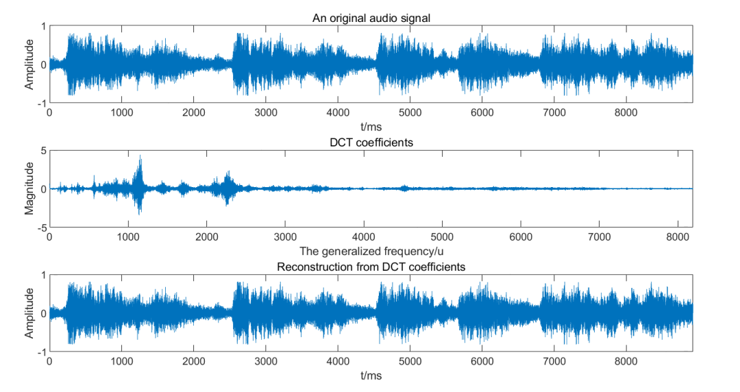 Figure 1 MATLAB Built-in Function DCT Result
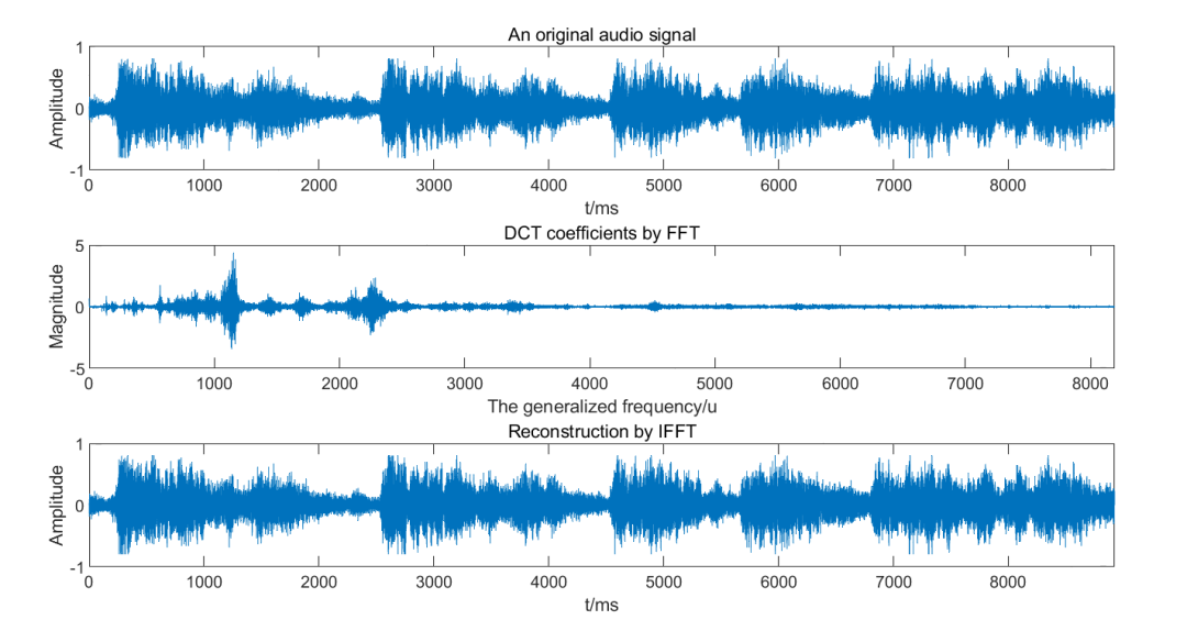 Figure 2 DCT Result Calculated Using FFT
The first half of the above code directly calls MATLAB’s built-in functions <span>dct</span> and <span>idct</span> to compute the results. The second half of the code implements decomposition and reconstruction based on the above principles using <span>fft</span> and <span>ifft</span>.
It can be seen that the results are consistent with those obtained by directly calling MATLAB’s built-in functions dct and idct. In fact, MATLAB’s built-in functions utilize FFT to implement DCT.
Appendix: LaTeX Code for Aligning Mathematical Formulas
Below is the LaTeX source code for the above formula (2), for reference and study.
$$
\begin{equation}
\label{eq.2}
\begin{aligned}
\ F_e(u)&=c(u)\displaystyle  \sum_{x=0}^{2N-1}f_e(x)cos \frac{(2x+1)u\pi}{2N}\\
&=c(u)\displaystyle \sum_{x=0}^{2N-1}f_e(x)Re\left[e^{-j\frac{(2x+1)u\pi}{2N}}\right]\\
&=c(u)Re\left[\displaystyle \sum_{x=0}^{2N-1}f_e(x)e^{-j\frac{(2x+1)u\pi}{2N}}\right]\\
& =c(u)Re\left[e^{-j\frac{u\pi}{2N}}\displaystyle \sum_{x=0}^{2N-1}f_e(x)e^{-j\frac{2xu\pi}{2N}}\right]
\end{aligned}
\end{equation}
$$
“The trivial and minute details that are often overlooked are the most substantial cornerstones embedded in learning and growth.”

Text and Images: Zhenming Peng
Editor: Simin LiuPrevious Issues Review
MATLAB Image Processing | Constructing Frequency Domain Filters from Spatial Domain Templates (Complete Code Included)
MATLAB Plotting Techniques | Setting Transparency of Color Bars (Complete Code Included)
MATLAB Plotting Techniques | Capturing Frames to Generate GIF Animations (Complete Code Included)
MATLAB Plotting Techniques | Standard Labeling of Graphs (With Example Code)
MATLAB Signal Simulation | In-depth Understanding of Frequency Resolution in Fourier Transform (With Example Code)
MATLAB Image Processing | Homomorphic Filtering of Grayscale Images (Complete Code Included)
MATLAB Plotting Techniques | Drawing Dual Y-axis Line Charts (With Example Code)
MATLAB Image Processing | Sigmoid Function Contrast Stretching (With Example Code)
MATLAB Plotting Techniques | Gamma Transformation Curve of Image Grayscale (With Example Code)
MATLAB Plotting Techniques | Clever Use of Graphics Handles (With Example Code)
MATLAB Plotting Techniques | Area Filling Between Two Lines with Color (With Source Code)
MATLAB Plotting Techniques | Fourier Series Expansion 3D Visualization Code Optimization
MATLAB Plotting Techniques | Data Visualization Color Schemes (With Code)
MATLAB Plotting Techniques | Pseudo-coloring of Grayscale Images (With Code)
MATLAB Plotting Techniques | Density Scatter Plot + Regression Line Removal (With Code)
MATLAB Plotting Techniques | 2D Scatter Plot (With Code)
MATLAB Plotting Techniques | 3D Curve Filling (With Code)
MATLAB Plotting Techniques | 3D Line Chart (With Code)
MATLAB Plotting Techniques | 3D Surface (With Code)
MATLAB Plotting Techniques | Custom Music Player (With Code)
MATLAB Plotting Techniques | Polygon Area Filling Chart (With Code)
MATLAB Plotting Techniques | Color Gradient Line Chart Drawing (With Code)
MATLAB Plotting Techniques | Line Chart Drawing (With Code)
MATLAB Plotting Techniques | Color Gradient Bar Chart Drawing
Sharing stories from life, discussing educational topics, chatting about the flavors of life, and writing words with warmth.