Follow+Star Public Number, Don’t Miss Exciting Content

Editor | strongerHuang
WeChat Public Account | Embedded Column
The principle of an oscilloscope is simply an ADC conversion, which displays the collected different voltages on the screen.
Today, we will discuss what the oscilloscope sampling rate is all about.
Example Describing Sampling Rate
1. Storage Depth
Imagine how to make a photo clear? Of course, the more pixels, the more original information the photo contains, making it closer to reality and naturally clearer.
The waveform we see on the oscilloscope can also be understood as a photo, and the more points this photo contains, the closer it is to the real appearance.
The storage depth of the oscilloscope indicates how many data points the oscilloscope can store at most. For example, a storage depth of 28Mpts means the oscilloscope can store up to twenty-eight million sampling points.
For taking a still photo, the speed of the camera shutter does not matter much, as the result will not change.
2. Sampling Rate
However, since signals are constantly changing, for an oscilloscope, it is more like continuously taking photos of moving objects at super high speeds. At this point, in addition to the number of sampling points, the speed at which the sampling points are collected is also crucial.
The oscilloscope’s reconstruction of a signal depends not only on how many data points there are but also on the speed of collecting those data points. The sampling rate of the oscilloscope is the capacity to collect how many data points per second. If the oscilloscope’s sampling rate is insufficient, we will not be able to accurately see the true appearance of the signal.
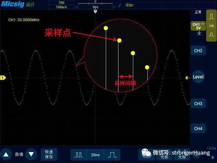
The input signal to the oscilloscope is continuously changing on both the time axis and the voltage axis. Since computers can only process discrete digital signals, such signals cannot be described and processed with digital methods. Therefore, a high-speed ADC is needed to sample and quantify the signal, which is the digitization process. After the Analog-to-Digital Conversion (ADC), the waveform that continuously changes in time and voltage becomes a series of continuously changing digital sampling points.
In the process of sampling or digital quantization, if we want to reconstruct the waveform as realistically as possible, the key issue is whether the sampling points on the time axis are dense enough and the quantization levels of the voltage in the vertical direction. The horizontal sampling point interval depends on the sampling rate of the oscilloscope’s ADC, while the vertical voltage quantization levels depend on the bit depth of the ADC.
The Operating Process of the Oscilloscope
The operating process of the oscilloscope is roughly as follows:
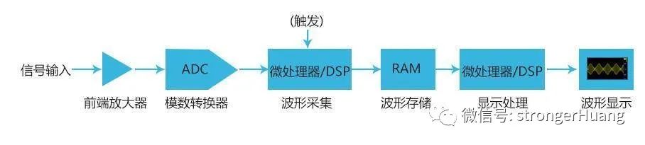
We input a signal to the oscilloscope via a probe. The measured signal passes through the oscilloscope’s front-end amplification/attenuation and other signal conditioning circuits, then goes to the high-speed ADC for signal sampling and digital quantization. The sampling rate of the oscilloscope is the frequency of the sampling clock during the Analog-to-Digital Conversion of the input signal, simply put, it is the sampling interval, with one sampling point collected per sampling interval.
For example, a sampling rate of 1GSa/s indicates that the oscilloscope has the capability to collect one billion sampling points per second, with a sampling interval of 1 nanosecond.
For real-time oscilloscopes, the commonly adopted method is real-time sampling.Real-time sampling means performing continuous high-speed sampling of the measured waveform signal at equal intervals and then reconstructing or restoring the waveform based on these continuous sampling points. A critical point in the real-time sampling process is to ensure that the oscilloscope’s sampling rate is much faster than the changes in the measured signal.
So how much faster should it be? You can refer to the Nyquist theorem in digital signal processing. The Nyquist theorem states that if the bandwidth of the measured signal is limited, then during sampling and quantization, if the sampling rate is more than twice the bandwidth of the measured signal, it is possible to fully reconstruct or restore the information contained in the signal without producing aliasing.
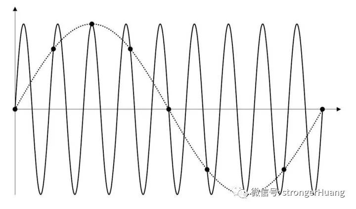
The following diagram shows the signal aliasing caused by insufficient sampling rate; you can see that the frequency of the collected signal has decreased significantly compared to the original signal.
Multiple Sampling Modes
Most oscilloscopes offer several sampling modes for users to choose from, commonly includingNormal Sampling, Average Sampling, Peak Sampling, and Envelope Sampling.
In normal sampling mode, the oscilloscope samples the signal at equal time intervals to reconstruct the waveform. This mode produces the best display effect for most waveforms.
In peak sampling mode, when the horizontal time base is set low, it retains the minimum and maximum sampling values to capture rare and narrow events (while amplifying any noise). This mode will display all pulses at least as wide as the sampling period. Peak sampling mode can be used to more conveniently view glitches or narrow pulses. In peak sampling mode, narrow glitches and rising edges appear brighter than in the ‘normal’ sampling mode, making them easier to see. Using peak sampling can avoid signal confusion but will also display more actual noise.
Using average sampling mode can average multiple acquisition results to reduce random or unrelated noise in the displayed signal. Averaging multiple sampling results requires stable triggering. The number of averages can be set in the selection box after the average sampling mode; the higher the number of averages, the slower the displayed waveform responds to waveform changes. A trade-off must be made between the response speed of the waveform to changes and the degree of noise reduction displayed on the signal.
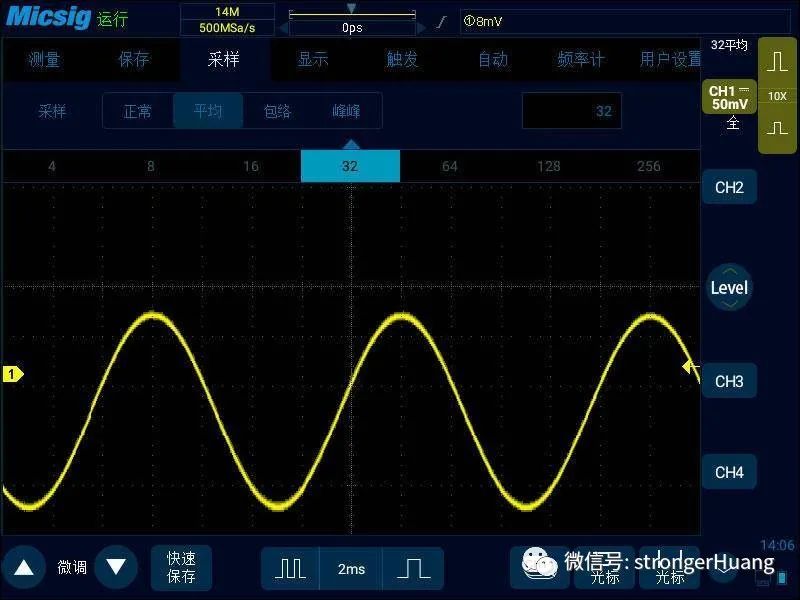
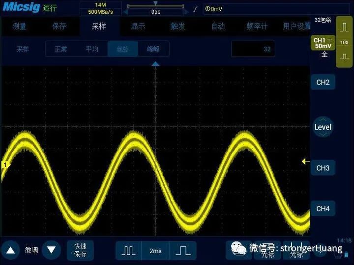
Using envelope sampling mode allows you to see the overlay effect of the waveforms sampled multiple times, capturing the maximum and minimum values of a signal within a specified number of sampling data. You can set the number of waveform overlays, as shown below for an amplitude-modulated signal with a waveform overlay count of 32 in envelope sampling mode.
No matter which sampling method is chosen, remember to ensure that the sampling rate is at least twice the bandwidth of the measured signal. In fact, we recommend at least 3-5 times higher, so that it is easier to capture abnormal information in the waveform.
One last thing worth noting is that the sampling rate of the oscilloscope is different from the bandwidth of the oscilloscope. When you open multiple channels, the sampling rate will be averaged across each channel. Therefore, if you open multiple channels, be sure to confirm again whether the sampling rate still meets the conditions.
Source: https://zhuanlan.zhihu.com/p/195535528
Disclaimer:This article’s materials are sourced from the internet, and the copyright belongs to the original author. If there are any copyright issues, please contact me for deletion.
———— END ————
Reply ‘ Science Popularization Knowledge ‘ or ‘ Microcontroller ‘ to read more related articles.
Welcome to follow my public account, reply ‘ Join Group ‘ to join the technical exchange group according to the rules, reply ‘ 1024 ‘ to see more content.Welcome to follow my video account:

Click ‘ Read Original ‘ to see more shares, and feel free to share, bookmark, like, and view.