Full text link: http://tecdat.cn/?p=4305
This example explores how to use a multifactor copula model to simulate correlated counterparty defaults. (Click “Read the original text” at the end for the complete code data).
Modeling Correlated Defaults with Copula
Related Video
Given the exposure to default risk, default probabilities, and loss given default information, estimate the potential loss of a counterparty portfolio. A Copula object is used for each debtor’s credit with a latent variable model. The latent variables consist of a series of weighted latent credit factors and each debtor’s specific credit factors. The latent variables are mapped to the default or non-default state of each debtor in each scenario based on their default probabilities. The Copula object supports portfolio risk measures, counterparty-level risk contributions, and simulation convergence information.
This example also explores the sensitivity of risk measures to the type of copula used for simulation (Gaussian copula vs. t copula).
Loading and Checking Portfolio Data
The portfolio contains 100 counterparties and their associated credit risk exposures (Exposure at Default – EAD), default probabilities (PD), and loss given default (LGD). Using the Copula object, you can simulate defaults and losses over a fixed time period (e.g., one year).
In this example, each counterparty is mapped to two underlying credit factors using a set of weights. The Weights2F variable is a matrix where each row contains the weights for a single counterparty. The first two columns are the weights for the two credit factors, and the last column is the specific weight for each counterparty. This example also provides the correlation matrix for the two underlying factors.
Loading Portfolio Information
Initialize the object using the portfolio information and factor correlations.
rng('default');
cc = creditDefaultCopula(EAD, PD, LGD, Weights2F, 'FactorCorrelation', FactorCorr2F);

cc.VaRLevel = 0.99;
DISP(cc)
creditDefaultCopula with properties:

    FactorCorrelation: [2x2 double]
    VaRLevel: 0.9900
    PortfolioLosses: []
cc.Portfolio(1:5,:)
ans =
    5x5 table
    ID      EAD      PD      LGD      Weight
    __    ______    _________    ____    ____________________
    1     121.6270    0.0050    0.350    0.3500    0.65
    2     23.2595     0.0601    0.350    0.4500    0.55
    3     320.3910    0.1101    0.550    0.1500    0.85
    4     43.7534     0.0020    0.250    0.3500    0.75
    5     55.7193     0.0601    0.350    0.3500    0.65
Simulating the Model and Plotting Potential Losses
Simulate the multifactor model. By default, the Gaussian copula is used. This function internally maps the implemented latent variables to default states and calculates the corresponding losses.
cc = simulate(cc, 1e5);
DISP(cc)
creditDefaultCopula with properties:

    FactorCorrelation: [2x2 double]
    VaRLevel: 0.9900
    PortfolioLosses: [1x100000 double]
The function returns risk measures and confidence intervals for the total portfolio loss distribution. The VaRLevel reports the Value at Risk (VaR) and Conditional Value at Risk (CVaR).
[pr, pr_ci] = portfolioRisk(cc);
fprintf('Portfolio risk metrics:\n');
DISP(pr);
fprintf('\n\nConfidence intervals for risk measures:\n');
DISP(pr_ci)
Portfolio risk metrics
    EL      Std      VaR      CVaR
    ______    ______    ______    ______
    24.774    23.693    101.57    120.22
Confidence intervals for risk measures:
    EL      Std      VaR      CVaR
    ____________________    ________________    ________________    ________________
    24.627    24.92    23.589    23.797    100.65    102.82    119.1    121.35
Examine the distribution of portfolio losses. Expected Loss (EL), VaR, and CVaR are marked as vertical lines. The economic capital indicated by the difference between VaR and EL is shown as the shaded area between EL and VaR.
plotline = @(x, color) plot([x x], ylim, 'LineWidth', 2, 'Color', color);

cvarline = plotline(pr.CVaR, 'm');
% Shade the area for expected loss and economic capital.
plotband = @(x, color) patch([x fliplr(x)], [0 0 repmat(max(ylim), 1, 2)],...
color, 'FaceAlpha', 0.15);
elband = plotband([0 pr.EL], 'blue');
ulband = plotband([pr.EL pr.VaR], 'red');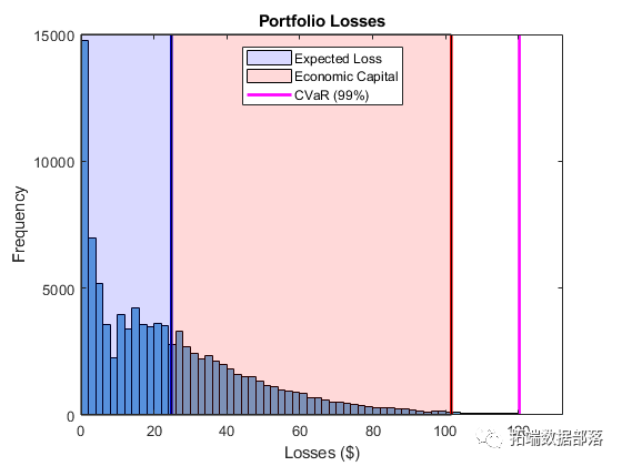
Click the title to view past content

[Video] Copula Algorithm Principles and Visualization Analysis of Stock Market Return Dependencies in R

Swipe left to see more
01
02
03
04
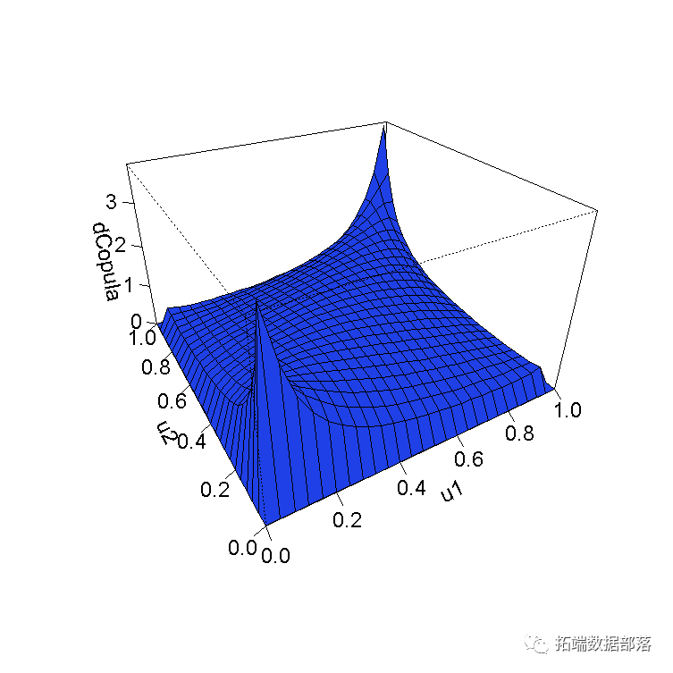
Identifying Concentration Risk of Counterparties
Use the riskContribution function to find the concentration risk in the portfolio. riskContribution returns each counterparty’s contribution to the portfolio’s EL and CVaR. These additional value contributions are summed with the corresponding total portfolio risk measures.
rc = riskContribution(cc);
% Report the percentage contribution of EL and CVaR.
rc(1:5,:)
ans =
    5x5 table
    ID      EL      Std      VaR      CVaR
    __    _________    __________    _______    _________
    1     10.0386    0.02495    0.10482    0.12868
    2     20.0670    0.036472    0.17378    0.24527
    3     1.2527    0.62684    2.0384    2.3103
    4     0.0023253    0.00073407    0.0026274
    5     0.11766    0.042185    0.27028    0.26223
Identifying the Counterparties with the Highest Risk through CVaR Contribution
[rc_sorted, idx] = sortrows(rc, 'CVaR', 'descend');
rc_sorted(1:5,:)
ans =
    5x5 table
    ID      EL      Std      VaR      CVaR
    __    _______    ______    ______    ______
    1     89      2.261    2.2158    8.1095    9.2257
    2     22      1.5672    1.8293    6.275    7.4602
    3     66      0.85227    1.4063    6.3827    7.2691
    4     16      1.6236    1.5011    5.8949    7.1083
Plot the counterparty risk and CVaR contributions. Counterparties with the highest CVaR contributions are plotted in red and orange.
pointSize = 50;
colorVector = rc_sorted.CVaR;
scatter(cc.Portfolio(idx,:).EAD, rc_sorted.CVaR,...
pointSize, colorVector, 'filled')
colormap('jet')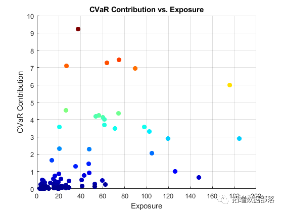
Studying Simulation Convergence with Confidence Bands
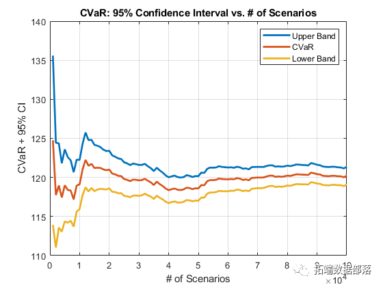
Investigate the convergence of the simulation. By default, the CVaR confidence intervals are reported, but optional RiskMeasure parameters support confidence intervals for all risk measures.
cb = confidenceBands(cc);
% Confidence bands are stored in a table.
cb(1:5,:)
ans =
    5x4 table
    NumScenarios    Lower    CVaR    Upper
    ______________    ______    ______    ______
    1000            113.92    124.76    135.59
    2000            111.02    117.74    124.45
    3000            113.58    118.97    124.36
    4000            113.06    117.44    121.81
    5000            114.38    118.99    123.6
Plot the confidence intervals to observe the speed of convergence of the estimates.
Obtain specific confidence intervals.
width = (cb.Upper - cb.Lower) ./ cb.CVaR;

plot(cb.NumScenarios, width * 100, 'LineWidth', 2);

% Find the confidence band at
% the 1% (two-sided) range of CVaR.
thresh = 0.02;
scenIdx = find(width <= thresh, 1, 'first');
scenValue = cb.NumScenarios(scenIdx);
widthValue = width(scenIdx);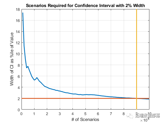
Comparing Tail Risks of Gaussian and t Copulas
Using a t copula increases the default correlation between counterparties. This leads to a more severe tail distribution of portfolio losses and results in higher potential losses.
cc_t = simulate(cc, 1e5, 'Copula', 't');
pr_t = portfolioRisk(cc_t);
% Understand how portfolio risk changes with t copula.

% Portfolio risk with Gaussian copula:
EL      Std      VaR      CVaR
______    ______    ______    ______
24.774    23.693    101.57    120.22
% Portfolio risk with t copula (dof = 5):
EL      Std      VaR      CVaR
______    ______    ______    ______
24.924    38.982    186.33    251.38
Compare the tail losses of each model.
Using a t copula with five degrees of freedom results in significantly higher tail risk measures for VaR and CVaR. The default correlation of t copulas is higher, leading to more instances of multiple counterparties defaulting. The number of degrees of freedom plays a crucial role. For very high degrees of freedom, the results using a t copula are similar to those using a Gaussian copula. For very low degrees of freedom, the results show significant differences. Furthermore, these results emphasize that the likelihood of extreme losses is highly sensitive to the choice of copula and the number of degrees of freedom.

The data and code analyzed in this article are shared in the member group. Scan the QR code below to join the group!


Click at the end of the article“Read the original text”
to obtain the complete data.
This article is excerpted from Using Copula for Simulating and Optimizing Market Risk Data VaR Analysis in MATLAB.

Click the title to view past content
R Language ARMA GARCH COPULA Model Fitting Stock Return Time Series and Simulation VisualizationARMA-GARCH-COPULA Model and Financial Time Series CaseTime Series Analysis: ARIMA GARCH Model Analysis of Stock Price DataGJR-GARCH and GARCH Volatility Forecasting for the S&P Index Time Series and Mincer Zarnowitz Regression, DM Test, JB Test[Video] Time Series Analysis: ARIMA-ARCH / GARCH Model Analysis of Stock PricesTime Series GARCH Model Analysis of Stock Market VolatilityPython GARCH, Discrete Stochastic Volatility Model DSV Simulation Estimation of Stock Return Time Series and Monte Carlo VisualizationExtreme Value Theory EVT, POT Over-threshold, GARCH Model Analysis of Stock Index VaR, Conditional CVaR: Diversified Portfolio Risk Measure AnalysisGARCH Volatility Forecasting Regime Switching Trading StrategyFinancial Time Series Models ARIMA and GARCH in Stock Market Forecasting ApplicationsTime Series Analysis Models: ARIMA-ARCH / GARCH Model Analysis of Stock PricesR Language Risk Value: ARIMA, GARCH, Delta-normal Method Rolling Estimation of VaR (Value at Risk) and Backtesting Analysis of Stock DataR Language GARCH Modeling Common Software Package Comparison, Fitting S&P 500 Index Volatility Time Series and Forecasting VisualizationPython Financial Time Series Models ARIMA and GARCH in Stock Market Forecasting ApplicationsMATLAB GARCH Model Fitting and Forecasting of Stock Market Return Time Series VolatilityR Language GARCH-DCC Model and DCC (MVT) Modeling EstimationPython ARIMA, GARCH Model Forecasting Analysis of Stock Market Return Time SeriesR Language Time Series Analysis Models: ARIMA-ARCH / GARCH Model Analysis of Stock PricesR Language ARIMA-GARCH Volatility Model Forecasting Stock Market Apple Inc. Daily Return Time SeriesPython GARCH, EGARCH, GJR-GARCH Models and Monte Carlo Simulation for Stock Price ForecastingR Language Time Series GARCH Model Analysis of Stock Market VolatilityR Language ARMA-EGARCH Model, Ensemble Forecasting Algorithm for SPX Actual Volatility ForecastingMATLAB Implementation of MCMC Markov Switching ARMA – GARCH Model EstimationPython GARCH, EGARCH, GJR-GARCH Models and Monte Carlo Simulation for Stock Price ForecastingUsing R Language for ARIMA + GARCH Trading Strategy on S&P 500 Stock IndexR Language Multivariate ARMA, GARCH, EWMA, ETS, Stochastic Volatility SV Model for Financial Time Series Data ModelingR Language Stock Market Index: ARMA-GARCH Model and Exploratory Analysis of Log Returns DataR Language Multivariate Copula GARCH Model Time Series ForecastingR Language Using Multivariate AR-GARCH Model to Measure Market RiskR Language Time Series Analysis Models: ARIMA-ARCH / GARCH Model Analysis of Stock PricesR Language Analyzing Stock Prices with GARCH Model and Regression ModelsComparison of VaR using GARCH (1,1), MA and Historical Simulation MethodMATLAB Estimation of ARMA GARCH Conditional Mean and Variance ModelsR Language POT Over-threshold Model and Extreme Value Theory EVT Analysis