Please respect the original work.Please indicate the link to this article.And the author of the article: slandarer
Everyone is familiar with infectious disease models. So, assuming we already have statistical data for S, I, and R, how do we determine the parameters? Before discussing this, let’s briefly describe the SIR model for infectious diseases:
Overview of Infectious Disease Models
S represents the susceptible individuals, I represents the infected individuals, and R represents the recovered individuals who will not get infected again. Susceptible individuals have a probability of becoming infected after contact with infected individuals, and infected individuals have a probability of recovering and becoming recovered individuals:
The rate of increase of infected individuals is related to both the number of infected individuals and the number of susceptible individuals, while the rate of change of recovered individuals only depends on the number of infected individuals.
To convert the discrete problem into a continuous one and to reduce the number of parameters to be determined, we will nondimensionalize the model (which means converting the units from number of individuals to percentages). Here, we will not consider deaths (the model considering deaths is left as an exercise~), assuming the total population is :
Thus, the total population remains unchanged, and we can perform the following nondimensionalization:
Substituting into the previous system of differential equations gives:
where , so we only have one parameter to determine.
Experimental Data
To conduct the experiment, we randomly generated a set of data: here is written as r0 to distinguish it from the initial proportion of recovered individuals : we set to 5 and added noise interference, generating the following experimental data:
%% Data Generation
S0 = 99/100;                % Initial proportion of susceptibles
I0 = 1/100;                 % Initial proportion of infected
R0 = 0;                     % Initial proportion of recovered
y0 = [S0, I0, R0];
r0 = 5;

% S = y(1), I = y(2)
sir_model = @(t, y, r0) [
   - r0*y(1)*y(2);          % dS/dt
     r0*y(1)*y(2) - y(2);   % dI/dt
     y(2);                  % dR/dt
];

exp_t = linspace(0, 10, 101).';
[sim_t, sim_y] = ode45(@(t, y) ...
    sir_model(t, y, r0), exp_t, y0);
sim_y = sim_y + (rand(size(sim_y)) - .5).*.05;  % Add noise interference
sim_y(sim_y < 0) = 0;
sim_y = sim_y./sum(sim_y, 2);

exp_S = sim_y(:,1);
exp_I = sim_y(:,2);
exp_R = sim_y(:,3);
save experimental_data_SIR_nondim exp_S exp_I exp_R exp_t
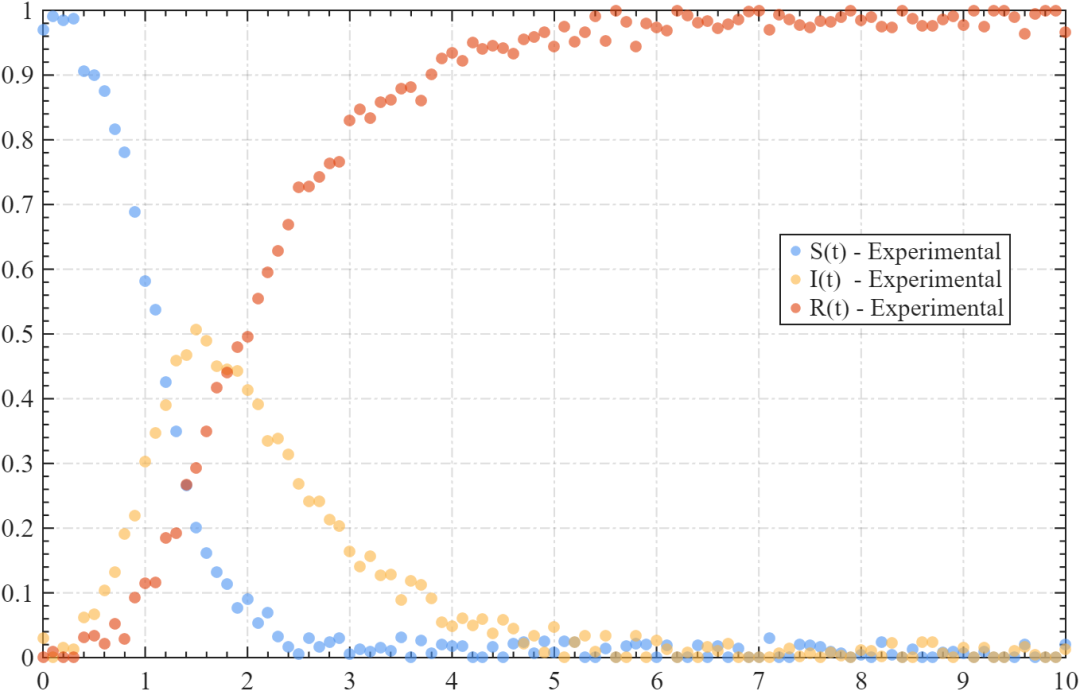
This data can be imported as follows:
% Data Import
SIRVD_data = load('experimental_data_SIR_nondim.mat');
exp_t = SIRVD_data.exp_t;
exp_S = SIRVD_data.exp_S;
exp_I = SIRVD_data.exp_I;
exp_R = SIRVD_data.exp_R;
disp('Experimental data loaded successfully from .mat files.');
Least Squares Estimation
The idea is very simple. We set and the initial data, use the Runge-Kutta method for simulation, and then try to find the that minimizes the difference between the simulated data and the real data, i.e.,
This objective function can be written in many ways; here are two methods:
Objective Function One
Where the <span>simulate_SIR</span> function uses the set for data simulation, and the <span>objective</span> compares the simulated data with the real data, which is quite clear:
% Objective Function Method One
function outputs = simulate_SIR(t_data, y0, r0, tspan, var_type)
    [t_sim, y_sim] = ode45(@(t, y) [
        - r0*y(1)*y(2);          % dS/dt
          r0*y(1)*y(2) - y(2);   % dI/dt
          y(2);                  % dR/dt
    ], tspan, y0);
    y_interp = interp1(t_sim, y_sim, t_data, 'linear', 'extrap');
    switch var_type
        case"S", outputs = y_interp(:, 1);
        case"I", outputs = y_interp(:, 2);
        case"R", outputs = y_interp(:, 3);
    end
end
objective = @(params, t_data, S_data, I_data, R_data, y0, tspan) ...
    sum((S_data - simulate_SIR(t_data, y0, params, tspan, "S")).^2) + ...
    sum((I_data - simulate_SIR(t_data, y0, params, tspan, "I")).^2) + ...
    sum((R_data - simulate_SIR(t_data, y0, params, tspan, "R")).^2);
This method is very clear, but it will call the <span>simulate_SIR</span> function many times. Additionally, if MATLAB is an older version, please place the <span>simulate_SIR</span> function at the end of the m file.
Objective Function Two
This method is more efficient, as it concatenates the three sets of SIR data for least squares:
% Objective Function Method Two
function y_interp = simulate_SIR(t_data, y0, r0, tspan)
    [t_sim, y_sim] = ode45(@(t, y) [
        - r0*y(1)*y(2);          % dS/dt
          r0*y(1)*y(2) - y(2);   % dI/dt
          y(2);                  % dR/dt
    ], tspan, y0);
    y_interp = interp1(t_sim, y_sim, t_data, 'linear', 'extrap');
end
objective = @(params, t_data, S_data, I_data, R_data, y0, tspan) ...
    sum(sum(([S_data, I_data, R_data] - simulate_SIR(t_data, y0, params, tspan)).^2));
Parameter Determination
Simply use MATLAB’s built-in <span>fminsearch</span> function:
% Use fminsearch function to find the R_0 that minimizes the difference between experimental and real values
S0 = 99/100;                % Initial proportion of susceptibles
I0 = 1/100;                 % Initial proportion of infected
R0 = 0;                     % Initial proportion of recovered
y0 = [S0, I0, R0];
r0_guess = 1;               % Guessed R0 (arbitrarily set initial value)
tspan = linspace(min(exp_t), max(exp_t), length(exp_t));
params_fit = fminsearch(@(params) objective(params, exp_t, exp_S, exp_I, exp_R, y0, tspan), r0_guess);
disp(['Estimated R0: ', num2str(params_fit(1))]);
The calculated value is quite accurate.
Plotting
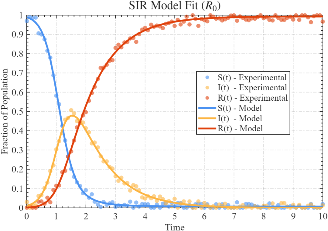
Let’s plot to show the fitting effect:
figure('Units','normalized', 'Position',[0,.4,.5,.5]);
axes('Parent',gcf, 'NextPlot','add');
% Palette
CList = [75,146,241; 252,180,65; 224,64,10; 5,100,146; 170,170,170]./255;
% Plot real data
scatter(exp_t, exp_S, 50, CList(1,:), 'filled', ...
    'MarkerFaceAlpha',.6, 'DisplayName', 'S(t) - Experimental');
scatter(exp_t, exp_I, 50, CList(2,:), 'filled', ...
    'MarkerFaceAlpha',.6, 'DisplayName', 'I(t)  - Experimental');
scatter(exp_t, exp_R, 50, CList(3,:), 'filled', ...
    'MarkerFaceAlpha',.6, 'DisplayName', 'R(t) - Experimental');
% Plot fitted data
plot(sim_t, sim_y(:, 1), 'Color',CList(1,:), ...
    'LineWidth', 3, 'DisplayName', 'S(t) - Model');
plot(sim_t, sim_y(:, 2), 'Color',CList(2,:), ...
    'LineWidth', 3, 'DisplayName', 'I(t)  - Model');
plot(sim_t, sim_y(:, 3), 'Color',CList(3,:), ...
    'LineWidth', 3, 'DisplayName', 'R(t) - Model');
% Image decoration
set(gca, 'Box', 'on', 'LineWidth',1, 'FontName','Times New Roman', ...
    'FontSize',16, 'XMinorTick','on', 'YMinorTick','on', ...
    'XGrid','on', 'YGrid','on', 'GridLineStyle','-.')
xlabel('Time', 'FontSize', 16);
ylabel('Fraction of Population', 'FontSize', 16);
title('SIR Model Fit ($R_0$)',...
    'FontSize', 20, 'Interpreter','latex');
legend('FontSize', 15, 'Location', 'best');
The effect is quite good:
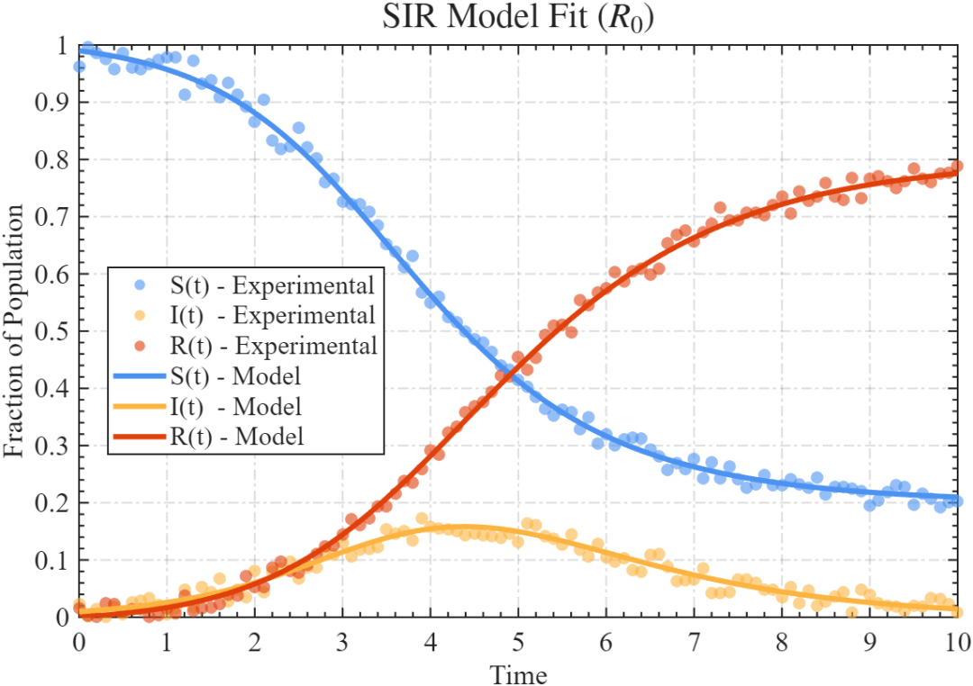
We can generate some other data, for example, when is 2, the fitting effect:
Approximate Bayesian Computation (ABC)
The name is quite interesting, abbreviated as the ABC method. The essence of this method is as follows:
Where represents our real data. If we set to a uniform distribution, we can use to estimate the possible distribution of parameters under the real data.
The idea of using this method is also simple. We randomly generate a bunch of within a certain range, obtain simulated data, and check the difference between each set of simulated data and the real values. If the difference is within an acceptable range, we store this . After storing a certain amount of (for example, 1000), we take the average of all stored values:
% Data Import
SIRVD_data = load('experimental_data_SIR_nondim.mat');
exp_t = SIRVD_data.exp_t;
exp_S = SIRVD_data.exp_S;
exp_I = SIRVD_data.exp_I;
exp_R = SIRVD_data.exp_R;
disp('Experimental data loaded successfully from .mat files.');

S0 = 99/100;                % Initial proportion of susceptibles
I0 = 1/100;                 % Initial proportion of infected
R0 = 0;                     % Initial proportion of recovered
y0 = [S0, I0, R0];
tspan = linspace(min(exp_t), max(exp_t), length(exp_t));
% S = y(1), I = y(2)
sir_model = @(t, y, r0) [
   - r0*y(1)*y(2);          % dS/dt
     r0*y(1)*y(2) - y(2);   % dI/dt
     y(2);                  % dR/dt
];


% ABC Method
N = 1000;                      % Number of accepted R_0 samples
accepted_samples = zeros(N,1); % Array to store accepted R_0 samples
threshold = 0.001;             % Acceptable error
r0_prior = [2, 8];             % Estimated range of R_0


fprintf('\r')
disp(['ABC sampling for threshold = ', num2str(threshold)])
disp('  0% ------------------------------ 100%')
fprintf('PROG ')
len_samples = 0;
while len_samples < N
    % Generate random R_0
    r0_sample = rand() * diff(r0_prior) + r0_prior(1);

    % SIR model Runge-Kutta simulation
    [~, y_sim] = ode45(@(t, y) ...
        sir_model(t, y, r0_sample), tspan, y0);
y_sim_S = interp1(tspan, y_sim(:, 1), exp_t, 'linear', 'extrap');
y_sim_I = interp1(tspan, y_sim(:, 2), exp_t, 'linear', 'extrap');
y_sim_R = interp1(tspan, y_sim(:, 3), exp_t, 'linear', 'extrap');

    % Calculate the mean difference between fitted data and real data
    distance = mean((exp_S - y_sim_S(:)).^2 + ...
                    (exp_I - y_sim_I(:)).^2 + ...
                    (exp_R - y_sim_R(:)).^2);

    % If the mean is less than the threshold, accept it
    if distance < threshold
        len_samples = len_samples + 1;
        if floor(30*len_samples/N) > floor(30*(len_samples - 1)/N)
            fprintf('#')
        end
        accepted_samples(len_samples) = r0_sample;
    end
end; fprintf(' END\r\n')

mean_r0 = mean(accepted_samples(:, 1), 1);  % Mean of accepted R0
std_r0 = std(accepted_samples(:, 1), 0, 1); % Standard deviation of accepted R0
disp(['Mean R0: ', num2str(mean_r0(1)), ', Std R0: ', num2str(std_r0(1))]);
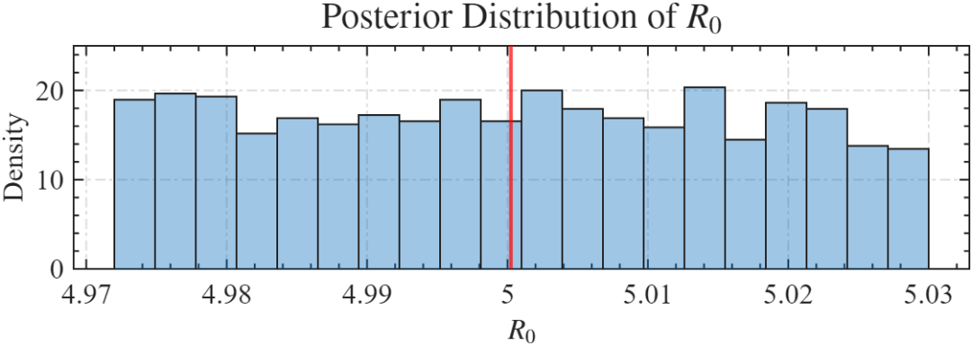
The smaller the allowable error, the more accurate the result, but it will take longer. For example, when set to 0.001, the result is:
- Mean R0: 5.0136, Std R0: 0.13391
For example, when set to 0.0005, the result is:
- Mean R0: 5.0002, Std R0: 0.016529
Let’s plot:
% Plotting
figure('Units','normalized', 'Position',[0,.1,.5,.25]); axes('Parent',gcf, 'NextPlot','add');
histogram(accepted_samples(:, 1), 20, 'Normalization', 'pdf', 'FaceAlpha',.4, 'LineWidth',1);
set(gca, 'LineWidth',1, 'FontSize',16, 'Box','on', 'FontName','Times New Roman', ...
    'XMinorTick','on', 'YMinorTick','on', 'XGrid','on', 'YGrid','on', 'GridLineStyle','-.')
xlabel('$R_0$', 'FontSize', 16, 'Interpreter','latex');
ylabel('Density', 'FontSize', 16);
title('Posterior Distribution of $R_0$', 'FontSize', 20, 'Interpreter','latex');
xline(mean_r0(1), 'r', 'LineWidth', 2, 'DisplayName', 'Mean $R_0$', 'Interpreter','latex');
Quiz
Since you have learned the parameter estimation of the SIR model, the SIRVD model, which requires determining three parameters, should be easy for you:
Where:
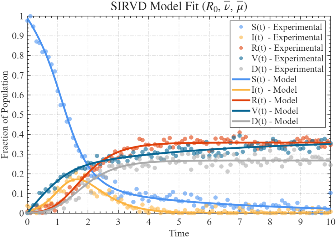
Let’s give it a try. I have placed the quiz questions and answers in the cloud drive~
- https://pan.baidu.com/s/193lmNOnoRzOLLupaeDJ0uQ?pwd=slan