What Is Monte Carlo Simulation?

Monte Carlo methods, also known as Monte Carlo experiments, are a collection of computational algorithms that rely on repeated random sampling to obtain numerical results. The basic concept is to use randomness to solve theoretically deterministic problems. These methods are often used to tackle physical and mathematical problems, and they can be particularly effective when faced with challenging issues. Monte Carlo methods are mainly used to solve three types of problems: optimization, numerical integration, and generating images based on probability distributions.

In physics-related problems, Monte Carlo methods can simulate systems with multiple coupled degrees of freedom, such as fluids, disordered materials, strongly coupled solids, and cellular structures (see Cellular Potts Model, Interacting Particle Systems, McKean-Vlasov Processes, Kinetic Models of Gases).

Other examples include modeling phenomena with significant uncertainty in inputs, such as risk calculations in business, and evaluating multidimensional integrals with complex boundary conditions in mathematics. In applications of systems engineering (space, oil exploration, aircraft design, etc.), Monte Carlo-based predictions of failures, cost overruns, and schedule overruns are often more effective than human intuition or other “soft” methods.

Theoretically, Monte Carlo methods can be used to solve any problem with a probabilistic interpretation. According to the Law of Large Numbers, an integral described by the expected value of a random variable can be approximated by the empirical mean (i.e., sample mean) of independent samples of that variable. When the probability distribution of the variable is parameterized, mathematicians often use Markov Chain Monte Carlo (MCMC) samplers. The central idea is to design an efficient Markov chain model with a given stationary probability distribution. That is to say, in the limit, the samples generated by the Markov Chain Monte Carlo method will become samples from the expected (target) distribution. Through the Ergodic Theorem, the stationary distribution can be approximated by the empirical measure of the random states of the Markov Chain Monte Carlo sampler.

In other problems, the goal is to generate images from sequences of probability distributions that satisfy nonlinear evolution equations. These probability distribution flows can always be interpreted as distributions of random states of a Markov process, where the transition probabilities depend on the distribution of the current random state (see McKean-Vlasov processes, Nonlinear Filtering Equations). In other cases, we have probability distribution flows with increasing sampling complexity (such as path space models with increasing time ranges, Boltzmann-Gibbs Measures related to decreasing temperature parameters, and many other examples). These models can also be viewed as the evolution of random state laws of a nonlinear Markov chain. A natural way to simulate these complex nonlinear Markov processes is to sample multiple copies of the process and use the empirical measure of the samples to replace the unknown random state distribution in the evolution equation. Compared to traditional Monte Carlo and Markov Chain Monte Carlo methods, these Mean Field Particle techniques rely on samples with continuous interactions. The term “mean field” reflects the fact that each sample (i.e., particle, individual, walker, medium, organism, or phenotype) interacts with the empirical measurement of the process. As the system size approaches infinity, these random empirical measures converge to the deterministic distribution of the random states of the nonlinear Markov chain, thereby eliminating statistical interactions between particles.

Despite the simplicity of its concepts and algorithms, the computational costs associated with Monte Carlo simulations can be astonishingly high. Generally, this method requires a large number of samples to achieve good approximations, and if the processing time for a single sample is long, it may lead to an overall run time that is difficult to control. Although this is a serious limitation in very complex problems, the embarrassingly parallel nature of the algorithm allows for reducing the high costs (perhaps to an acceptable level) through parallel computing strategies using local processors, clusters, cloud computing, GPUs, FPGAs, etc.

Overview

Monte Carlo methods differ widely, but tend to follow a specific pattern:

1. Define the domain of possible inputs

2. Randomly generate inputs from the probability distribution over the domain

3. Perform deterministic calculations on the inputs

4. Summarize the results

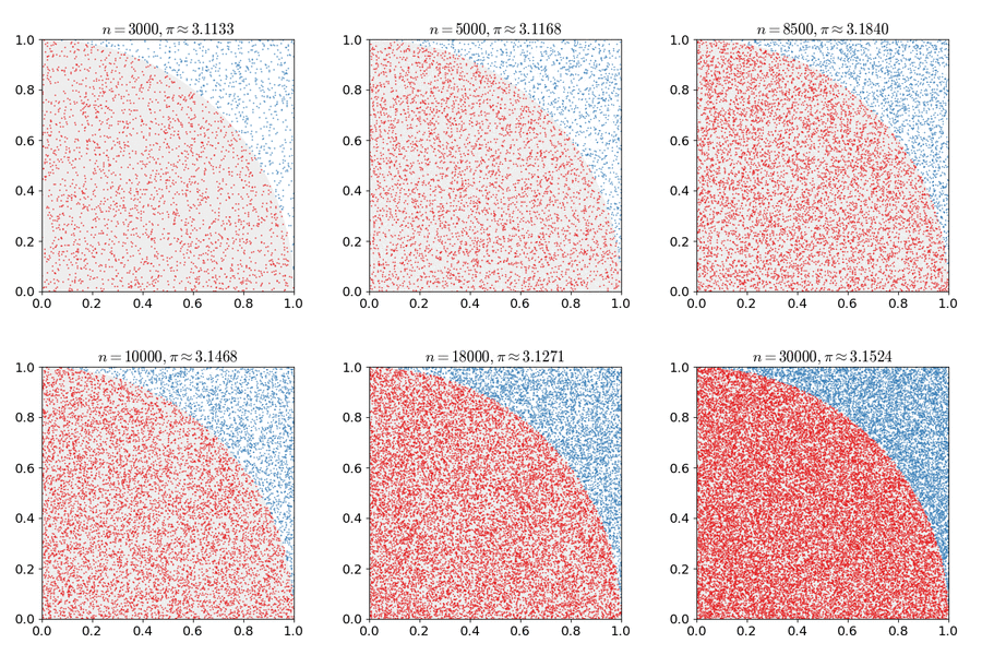
Monte Carlo methods applied to estimate the value of π.

For example, consider a quarter circle inscribed within a unit square. Given their area ratio is π/4, the value of π can be approximated using Monte Carlo methods:

1. Draw a square and then inscribe a quarter circle within it

2. Uniformly scatter a given number of points over the square

3. Count the number of points that fall within the quarter circle, i.e., those satisfying the condition of being less than 1 unit from the origin

4. The ratio of the count of points inside the quarter circle to the total sample count is an estimate of the ratio of the two areas, π/4. Multiply the result by 4 to estimate the value of π.

In this process, the input domain is the square that confines the quarter circle. We generate random inputs by scattering particles over the square and then perform calculations on each input (testing whether it is inside the quarter circle). Summarizing these results yields the final result—the approximate value of π.

There are two important considerations:

1. If these points are not uniformly distributed, the approximation will be poor.

2. This process requires a lot of points. If there are only a few randomly placed points in the entire square, this approximation is usually poor. On average, as more points are placed, the accuracy of the approximation increases.

Using the Monte Carlo method requires a large number of random numbers, which has stimulated the development of Pseudorandom Number Generators, which are much faster than the random number tables previously used for statistical sampling.

History

Before the development of Monte Carlo methods, people simulated tests of already solved deterministic problems by estimating uncertainties in simulations through statistical sampling. Monte Carlo simulation reverses this approach, using probabilistic metaheuristics to solve deterministic problems (see Simulated Annealing).

Early variants of Monte Carlo methods were designed to solve Buffon’s Needle Problem, where π can be estimated by dropping a needle onto a floor composed of parallel equidistant lines. In the 1930s, Enrico Fermi first experimented with the Monte Carlo method while studying neutron diffusion, but he did not publish this work.

In the late 1940s, Stanislaw Ulam invented the modern version of the Markov Chain Monte Carlo method while researching nuclear weapons projects at Los Alamos National Laboratory. Following Ulam’s breakthrough, John von Neumann immediately recognized its significance. Von Neumann programmed the ENIAC (the first electronic digital computer) to perform Monte Carlo calculations. In 1946, nuclear physicists at Los Alamos were studying neutron diffusion in fissionable materials. Despite having most of the necessary data, such as the average distance neutrons travel in matter before colliding with atomic nuclei and how much energy neutrons may release after collisions, they were unable to solve this problem using traditional deterministic mathematical methods. At this point, Ulam suggested using random experiments. He later recalled the inspiration process:

I initially conceived and attempted the Monte Carlo method in 1946, while I was recovering from an illness and often played solitaire. At that time, I pondered a question: what is the probability of successfully playing a game of 52-card Garfield? After spending a lot of time trying to estimate it through pure combinatorial calculations, I wondered if there was a more practical method than “abstract thinking,” possibly not unfolding it 100 times and simply observing and counting the number of successful games. With the advent of fast computers, this became imaginable, and I immediately thought of neutron diffusion and other mathematical physics problems, as well as the more general question—how to transform processes described by certain differential equations into equivalent forms that can be interpreted as a series of random operations. Later (in 1946), I described this idea to John von Neumann, and we began planning the actual calculations.

The work of von Neumann and Ulam was conducted in secrecy and required a code name. A colleague of von Neumann and Ulam, Nicholas Metropolis, suggested using the name Monte Carlo, which referred to the Monte Carlo casino in Monaco, where Ulam’s uncle would borrow money from relatives and then gamble. Using a list of “truly random” random numbers was extremely slow; however, von Neumann developed a method for generating pseudorandom numbers using the Middle-Square Method. Although many have criticized this method as being crude and primitive, von Neumann was aware of this: he demonstrated that this method was faster than any other method and pointed out that when it failed, it was easy to detect, unlike errors generated by other methods that might be difficult to notice.

Despite the severe limitations of the computing tools available at the time, Monte Carlo methods remained central to the simulations required by the Manhattan Project. In the 1950s, they were used in early work related to hydrogen bomb development at Los Alamos and became popular in the fields of physics, physical chemistry, and operations research. The RAND Corporation and the U.S. Air Force were the two main organizations responsible for funding and promoting information about Monte Carlo methods, and from that point on, they began to be widely applied in many different fields.

The theory of more complex mean-field type particle Monte Carlo methods emerged in the mid-1960s, initially stemming from a Markov interpretation of a class of nonlinear parabolic partial differential equations that appeared in fluid mechanics researched by Henry P. McKean Jr. Theodore E. Harris and Herman Kahn published a groundbreaking paper in 1951 that used mean-field genetic Monte Carlo methods to estimate energy transport in particles. This method has also been used as a heuristic natural search algorithm in evolutionary computation (also known as metaheuristics). The origins of these mean-field computational techniques can be traced back to 1950 and 1954 when Alan Turing worked on genotype mutation-selection learning machines, as well as articles by Nils Aall Barricelli from the Institute for Advanced Study in Princeton, New Jersey.

Quantum Monte Carlo methods, more specifically diffusion Monte Carlo methods, can also be interpreted as mean-field particle Monte Carlo approximations of Feynman-Kac path integrals. The origins of quantum Monte Carlo methods are typically attributed to Enrico Fermi and Robert Richtmyer, who developed the mean-field particle interpretation of neutron chain reactions in 1948. However, the first class of heuristic and genetic particle algorithms (also known as resampling or reconstruction Monte Carlo methods) used to estimate the ground state energy of quantum systems (in simplified matrix models) was proposed by Jack H. Hestirington in 1984. In molecular chemistry, the use of genetic heuristic particle methods (also known as reduction and enrichment strategies) can be traced back to the pioneering work of Marshall Rosenbluth and Arianna Rosenbluth in 1955.

Sequential Monte Carlo methods used in advanced signal processing and Bayesian inference have only emerged recently. In 1993, Gordon et al. published the first application of Monte Carlo resampling algorithms in Bayesian inference statistics in their groundbreaking work. The authors named their algorithm the “bootstrap filter” and demonstrated that their bootstrap filtering algorithm did not require any assumptions about the system state space or noise compared to other filtering methods. Additionally, Genki Kitagawa conducted pioneering research related to “Monte Carlo filters.” In the mid-1990s, Pierre Del Moral, Himilcon Carvalho, and Pierre Del Moral, André Monin, and Gérard Salut published articles on particle filters. Between 1989 and 1992, at LAAS-CNRS (Laboratory for Analysis and Architecture of Systems), Pierre Del Moral, J. C. Noyer, G. Rigal, and Gérard Salut developed particle filters for signal processing. They collaborated with STCAN (Department of Naval Construction and Armament Service Technology) and IT company DIGILOG to complete a series of restrictive and confidential research reports on radar/sonar and GPS signal processing issues. These sequential Monte Carlo methods can be interpreted as an acceptance-rejection sampler equipped with an interacting recycling mechanism.

From 1950 to 1996, all publications on sequential Monte Carlo methods, including those introducing reduction and resampling Monte Carlo methods in computational physics and molecular chemistry, currently apply to different situations with natural and heuristic algorithms without any consistency proofs or discussions of estimation bias and algorithms based on lineage and genetic trees. In his writings in 1996, Pierre Del Moral articulated the mathematical foundations of these particle algorithms and provided the first rigorous analysis of them.

In the late 1990s, Dan Crisan, Jessica Gaines, and Terry Lyons, along with Dan Crisan, Pierre Del Moral, and Terry Lyons, also developed branching particle methods with different population sizes. In 2000, Pierre Del Moral, Alice Guionnet, and Laurent Miclo further advanced this field.

Definition

There is no consensus on how to define Monte Carlo. For example, Ripley defines most probabilistic modeling as stochastic simulation, while Monte Carlo encompasses Monte Carlo integration and Monte Carlo statistical tests. Sawilowsky distinguishes simulation, Monte Carlo methods, and Monte Carlo simulations: simulation is a fictional representation of reality, Monte Carlo methods are techniques used to solve mathematical or statistical problems, and Monte Carlo simulation uses repeated sampling to obtain statistical characteristics of certain phenomena (or behaviors). For example:

Simulation: Drawing a pseudorandom uniform variable from the interval [0,1] can be used to simulate flipping a coin: if the value is less than or equal to 0.50, the result is heads; if the value is greater than 0.50, the result is tails. This is a simulation but not a Monte Carlo simulation.

Monte Carlo Method: Pouring a box of coins onto a table and then calculating the ratio of heads to tails. This is a Monte Carlo method of determining the outcome of repeated coin flips, but it is not a simulation.

Monte Carlo Simulation: Drawing “a large number” of pseudorandom uniform variables from the interval [0,1], assigning values less than or equal to 0.50 as heads and greater than 0.50 as tails. This is the behavior of a “Monte Carlo simulation” of multiple coin flips.

Kalos and Whitlock point out that the distinctions between these methods are not always easy to discern. For example, radiation from atoms is a natural random process. It can be directly simulated or described by random equations that capture its average behavior, and these random equations themselves can be solved using Monte Carlo methods. “In fact, the same computer code can simultaneously be viewed as ‘natural simulation’ or as solving equations through natural sampling.”The main idea of Monte Carlo and random numbers is based on repeated random sampling and statistical analysis to compute results. Monte Carlo simulation is, in fact, a form of random experiment, in which the outcomes of these experiments are unknown. A typical feature of Monte Carlo simulation is that there are many unknown parameters, many of which are difficult to obtain experimentally. The Monte Carlo simulation method does not always require truly random numbers to be useful (although unpredictability is crucial for some applications, such as prime testing). Many of the most useful techniques use deterministic pseudorandom sequences, making testing and rerunning simulations easier. Pseudorandom sequences are, in some sense, “random enough,” which is the only necessary property for conducting good simulations.The meaning of “random enough” generally depends on the application context but should typically be verified through a series of statistical tests. When the number of elements in the sequence to be considered is large enough, one of the simplest and most common ways to test whether these numbers are uniformly distributed or follow another expected distribution is to check for weak correlations between consecutive samples, which is often desirable or necessary.Sawilowsky listed the characteristics of high-quality Monte Carlo simulations:

The (pseudorandom number) generator has certain features (for example, the sequence has a long “period” before repeating)

The (pseudorandom number) generator can produce values that pass randomness tests

There are enough samples to ensure accurate results

Appropriate sampling methods are used

The algorithms used are effective for the modeling content

It can simulate phenomena in the problem

Pseudorandom Number Sampling Algorithms convert uniformly distributed pseudorandom numbers into numbers distributed according to a given probability distribution.Low-discrepancy sequences are often used instead of random sampling in space because they ensure uniform coverage and typically have faster convergence rates than Monte Carlo simulations that use random or pseudorandom sequences. Methods based on their use are referred to as Quasi-Monte Carlo Methods.To assess the impact of random number quality on Monte Carlo simulation results, astrophysicists tested cryptographically secure pseudorandom numbers generated by Intel’s RDRAND instruction set against pseudorandom numbers generated by the Mersenne Twister algorithm during the Monte Carlo simulation of brown dwarf radio flares. RDRAND is the closest pseudorandom number generator to a true random number generator. For trials generating 10 million random numbers, there was no statistical difference between the models generated by typical pseudorandom number generators and RDRAND.

Monte Carlo Simulation and “Hypothetical” Scenarios

Using probabilistic methods is not necessarily synonymous with Monte Carlo simulation—for example, deterministic modeling using point estimates. Each uncertain variable in the model is assigned a “best guess” estimate. Scenarios (such as best, worst, or most likely cases) are chosen for each input variable, and results are recorded.In contrast, Monte Carlo simulation samples each variable from probability distributions, producing hundreds or thousands of possible outcomes. An analysis of the results yields the probabilities of different outcomes occurring. For example, comparing an electronic spreadsheet cost modeling that runs under traditional “hypothetical” scenarios with Monte Carlo simulation and triangular probability distributions shows that the range of Monte Carlo analysis is narrower than that of “hypothetical” analysis. This is because “hypothetical” analysis gives equal weight to all scenarios (see quantifying uncertainty in corporate financing), while Monte Carlo methods sample very little in regions of very low probability. This portion of the sample is referred to as “rare events.”

Applications

Monte Carlo methods are particularly well-suited for simulating phenomena with significant uncertainty in input and multi-degree-of-freedom coupled systems. Application areas include:

Physical Sciences

Monte Carlo methods are very important in computational physics, physical chemistry, and related fields, with widespread applications ranging from complex Quantum Chromodynamics calculations to designing heat shields and aerodynamic forms, as well as simulating radiation transport in radiation dose calculations. In statistical physics, Monte Carlo molecular modeling is an alternative method for calculating molecular dynamics, where Monte Carlo methods are used to compute statistical field theories of simple particles and polymer systems. Quantum Monte Carlo methods address the many-body problem in quantum systems. In radiation materials science, simulating ion implantation using the binary collision approximation is often based on Monte Carlo methods to select the next collision atom. In experimental particle physics, Monte Carlo methods are used to design detectors, understand their behavior, and compare experimental data with theory. In astrophysics, they are used in various ways to simulate galaxy evolution and the transmission of microwave radiation through rough planetary surfaces. Monte Carlo methods also form the basis of ensemble models that constitute modern weather forecasting.

Engineering

Monte Carlo methods are widely used in sensitivity analysis in engineering design and quantitative probabilistic analysis in process design. This demand arises from the interactivity, collinearity, and nonlinear behavior typical of process simulations. For example:

In microelectronics engineering, Monte Carlo methods are used to analyze correlated and uncorrelated variations in analog and digital integrated circuits.
In geostatistics and geometallurgy, Monte Carlo methods form the basis for mineral processing flow design and assist in quantitative risk analysis.
In wind energy yield analysis, different uncertainties (P90, P50, etc.) are considered to calculate the predicted energy generation of wind farms over their lifecycle.
Simulating the impact of pollution and comparing diesel and gasoline.
In fluid dynamics, particularly rarefied gas dynamics, direct simulation Monte Carlo methods combined with efficient computational algorithms are used to solve the Boltzmann equation for fluids with finite Knudsen numbers.
In autonomous robotics, Monte Carlo localization can determine a robot’s position. It is commonly applied in random filters, such as Kalman filters or particle filters, forming the core of simultaneous localization and mapping (SLAM) algorithms.
In telecommunications, when planning wireless networks, it is necessary to demonstrate that designs are applicable for various scenarios involving different user numbers, user locations, and services they wish to use. Monte Carlo methods are often used to generate these users and their states. Network performance is then evaluated, and if the results are unsatisfactory, network design optimization is performed.
In reliability engineering, given component-level responses, Monte Carlo simulations are used to calculate system-level responses. For example, for a transportation network affected by seismic events, given the failure probabilities of its components, such as bridges and roads, Monte Carlo simulations can be used to assess the k-terminal reliability of the network. Another far-reaching example is applying Monte Carlo methods to solve G-update equations of the Generalized Renewal Process.
In signal processing and Bayesian inference, particle filters and sequential Monte Carlo techniques are a class of mean-field particle methods used for sampling and computing posterior distributions of signal processes given noise and local observations, using interacting empirical measures.
In groundwater simulation, Monte Carlo methods have generated a large number of realizations of heterogeneous parameter fields for model uncertainty quantification or parameter inversion.

C Climate Change and Radiative Forcing

The Intergovernmental Panel on Climate Change employs Monte Carlo methods to analyze probability density functions of radiative forcing.Effective Radiative Forcing (ERF) probability density functions are based on total greenhouse gases, aerosol forcing, and total anthropogenic forcing. Greenhouse gases consist of well-mixed greenhouse gases (WMGHG), ozone, and stratospheric water vapor. The probability density function is generated based on the uncertainties provided in Table 8.6. Using the method of Boucher and Haywood (2001), Monte Carlo simulations combine individual radiative forcing agents to derive the total forcing of the industrial era. The probability density function of effective radiative forcing from changes in ground albedo and mixed contrails and contrail-induced cirrus clouds is included in the total anthropogenic forcing rather than being displayed as independent probability density functions. We currently do not have effective radiative forcing estimates for some forcing mechanisms, such as ozone, land use, and solar energy.

Computational Biology

Monte Carlo methods are used across various fields of computational biology, such as Bayesian inference in phylogenetics or studying biological systems like genomes, proteins, or membranes. The system can be studied in a coarse-grained or ab initio computational framework, depending on the desired accuracy. Computer simulations allow us to monitor the local environment of specific molecules to see if a certain chemical reaction is occurring, for example. Thought experiments can be conducted in cases where physical experiments are not feasible (e.g., breaking bonds, introducing impurities at specific locations, altering local/global structures, or introducing external fields).

Computer Graphics

Path tracing, occasionally referred to as Monte Carlo ray tracing, presents a three-dimensional scene by randomly tracing possible light paths. Repeated sampling for any given pixel will ultimately lead to the average of the samples converging to the correct solution of the rendering equation, making it one of the most physically accurate 3D graphics rendering methods in existence.

Applied Statistics

The statistical standards of Monte Carlo methods were established by Sawilowsky. In applied statistics, Monte Carlo methods can be used for at least four purposes:1. Comparing competing statistics of small samples under real data conditions. Although asymptotic conditions of data based on classical theoretical distributions (e.g., normal curves, Cauchy distributions) can be computed for type I errors and statistical power characteristics, practical data often do not have such distributions.2. Providing implementations of hypothesis tests that are more effective than exact tests, such as permutation tests (which are often impossible to compute), while being more precise than asymptotic distribution critical values.3. Providing a random sample from posterior probabilities in Bayesian inference. All fundamental characteristics of the posterior can then be approximated and summarized based on this sample.4. Providing effective random estimates of the Hessian matrix of the negative log-likelihood function, which can form estimates of the Fisher Information matrix.Monte Carlo methods are also a compromise between approximate random and permutation tests. Approximate randomization tests are based on specific subsets of all permutations (which may require a lot of internal processing, with permutations taken into account). In contrast, Monte Carlo methods are based on a specified number of random permutations (if a permutation is drawn twice or more frequently, there is a slight loss of precision as it is unnecessary to track which permutations have already been selected).

Applications of Artificial Intelligence in Games

Monte Carlo methods have evolved into a technique known as Monte Carlo tree search, which can be used to search for the best moves in games. Possible moves are organized in a search tree, and many random simulations are used to estimate the long-term potential of each move. A black-box simulator represents the opponent’s actions.The Monte Carlo tree search (MCTS) method has four steps:1. Starting from the root node of the tree, select the best child node until reaching a leaf node.2. Expand the leaf node and select one of its child nodes.3. Play a simulated game starting from that node.4. Use the results of the simulated game to update the node and its ancestors.In many simulated games, the net effect is that a node representing a move will rise or fall in value, hopefully corresponding to the outcome of that node’s move (whether good or bad).Monte Carlo tree search has been successfully used in games like Go, Rainbow Chess, Battleship, and Indian Chaturanga.

Design and Visual Effects

Monte Carlo methods are also effective in solving integral differential equations of radiation fields and energy transport coupling, thus being used in global illumination computations to generate realistic virtual 3D model images, and are applied in video games, architecture, design, computer-generated films, and movie effects.Search and RescueThe U.S. Coast Guard uses Monte Carlo methods in its computer modeling software—Search and Rescue Optimal Planning System (SAROPS)—to calculate possible vessel locations during search and rescue operations. Each simulation can generate up to 10,000 data points that are randomly distributed based on provided variables. Search patterns are then inferred from this data to optimize probability of containment (POC) and probability of detection (POD), both of which together equal the overall success probability (POS). Ultimately, as a practical application of probability distribution, it aims to save lives and resources through the fastest and most convenient rescue methods.

Finance and Business

Monte Carlo simulations are commonly used to assess the risks and uncertainties affecting the outcomes of different decision-making scenarios. Monte Carlo simulations allow business risk analysts to incorporate the overall impact of uncertain variables, such as sales, commodity and labor prices, interest rates, and exchange rates, as well as the effects of different risk events, such as contract cancellations or changes in tax laws.In finance, Monte Carlo methods are frequently used to evaluate project investments at the business unit or company level, or other financial valuations. They can be used to simulate project timelines, where simulations aggregate estimates of worst-case, best-case, and most likely durations for each task to determine the overall project outcome. Monte Carlo methods are also used for option pricing, default risk analysis, and can be used to estimate the financial impact of medical interventions.

Law

Monte Carlo methods have been used to assess the potential value of a proposal aimed at helping women in Wisconsin successfully petition for harassment and domestic abuse restraining orders. By assisting women in completing petitions and providing them with more advocacy, it could potentially reduce the risk of rape and personal assaults. However, there are many variables that cannot be fully estimated, including the effectiveness of restraining orders, the success rates of petitioners, and many other factors. The study used experiments to alter these variables to provide an overall estimate of the program’s success.

Mathematical Applications

In general, Monte Carlo methods solve various problems in mathematics by generating suitable random numbers (see also random number generation) and observing numerical fractions that satisfy certain properties. This method is useful for problems that are too complex to solve analytically. The most common application of Monte Carlo methods is Monte Carlo integration.

Integration

Monte Carlo integration works by comparing random points and function values.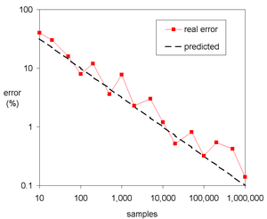Deterministic numerical integration algorithms work well in low dimensions but encounter two problems when the function has multiple variables. First, as the dimensionality increases, the number of function evaluations needed increases rapidly. For example, if 10 evaluations provide sufficient accuracy in one dimension, then 100 dimensions require 10¹⁰⁰ points, which is too many to compute. This is known as the Curse of Dimensionality. Second, the boundaries of multidimensional regions can be very complex, making it infeasible to simplify the problem to iterative integration. Problems in 100 dimensions are common because in many physical problems, one “dimension” corresponds to one degree of freedom.Monte Carlo methods provide a way to escape this exponential growth in computation time. As long as the function involved has reasonable properties, random points can be selected in a 100-dimensional space, and the average of some function values at these points can be used to estimate the integral. By the Central Limit Theorem, this method shows a 1/√N convergence, meaning that regardless of the dimensionality, doubling the number of sample points will halve the error.This method is improved in statistics and is called importance sampling, which involves randomly sampling points but more frequently where the integrand is larger. To do this accurately, the integral must be known, or it can be approximated using a similar function’s integral or through adaptive routines such as stratified sampling, recursive stratified sampling, adaptive umbrella sampling, or the VEGAS algorithm.A similar approach—quasi-Monte Carlo methods—uses low-discrepancy sequences. These sequences better “fill” the region, sampling more frequently at the most important points, and thus quasi-Monte Carlo methods often converge to the integral faster than Monte Carlo simulations using random or pseudorandom sequences.Another class of sampling point methods in volume is simulating random walks on it (Markov Chain Monte Carlo). These methods include the Metropolis-Hastings Algorithm, Gibbs Sampling, Wang and Landau Algorithm, and interactive Markov Chain Monte Carlo methods, such as Sequential Monte Carlo Sampling.

Simulation and Optimization

Random numbers have another powerful and very popular application in numerical simulation for numerical optimization. The problem is to minimize (or maximize) a function of certain vectors, which often have multiple dimensions. Many problems can be framed this way: for example, a computer chess program can be viewed as trying to find a set of moves, say, the 10 moves that yield the best evaluation function at the end. In the traveling salesman problem, the goal is to minimize the travel distance. There are also applications in engineering design, such as multi-disciplinary design optimization (MDO). It has also been applied to quasi-one-dimensional models to solve particle dynamics problems, effectively exploring large configuration spaces. References provide a comprehensive review of many issues related to simulation and optimization.The traveling salesman problem is referred to as a traditional optimization problem. That is, all the facts required to determine the optimal path (the distance between each destination) are certain, and the goal is to derive the path that minimizes the total distance of possible travel options. However, suppose we do not want to minimize the total distance required to visit each desired destination but instead minimize the total time required to reach each destination. This transcends traditional optimization because travel time is inherently uncertain (traffic congestion, time of day, etc.). Therefore, to determine our optimal path, we need to use simulation optimization to first understand the range of time that may be required to travel from one point to another (represented in this example by probability distributions rather than specific distances), and then optimize our travel decisions to determine the best path considering this uncertainty.

Inverse Problems

The probabilistic formulation of inverse problems leads to the definition of probability distributions in model space. This probability distribution combines prior information with new information obtained by measuring some observable parameters (data). Since in general, the theory that links data to model parameters is nonlinear, posterior probabilities in model space may not be easily described (they may be multimodal, and some moments may not be defined, etc.).When analyzing inverse problems, obtaining the maximum likelihood model is often not sufficient, as we typically also want information about data resolution. In general, we may have many model parameters, and testing the marginal probability density may be impractical or even useless. However, a large number of models can be pseudorandomly generated based on the posterior probability distribution and analyzed and displayed in a manner that conveys relative likelihood information about the model properties. This can be accomplished through an efficient Monte Carlo method, even in the absence of explicit formulas for prior distributions.The most famous importance sampling method, the Metropolis-Hastings algorithm, can be generalized to provide a method that allows analysis (possibly highly nonlinear) of inverse problems with complex prior information and arbitrary noise distribution data.

Philosophy

McCracken has extensively elucidated the Monte Carlo method. Elishakoff, Grüne-Yanoff, and Weurich discuss the general philosophy of the method.

Editor’s Recommendation

Course Recommendations

Unveiling AlphaGo: Deep Reinforcement Learning and Monte Carlo Search

https://campus.swarma.org/course/177

Arguably, AlphaGo marks the pinnacle of modern artificial intelligence technology, with its core algorithms being twofold: deep reinforcement learning and Monte Carlo search. Deep reinforcement learning is a blend of deep learning techniques and ancient reinforcement learning techniques; Monte Carlo search is a fast search algorithm that completes moves through simulated matches. AlphaGo skillfully integrates deep reinforcement learning, Monte Carlo search, and other technologies to achieve a significant advancement in the history of artificial intelligence. This course will provide a comprehensive interpretation of the deep learning technology behind AlphaGo.

Monte Carlo Methods

https://campus.swarma.org/course/552Monte Carlo methods, also known as computer random simulation methods, are a computational method based on “random numbers.” Monte Carlo methods differ significantly from general computational methods, which find it very challenging to solve multidimensional or complex factor problems, while Monte Carlo methods simplify solving such problems by cleverly using the “frequency” of event occurrences to determine the “probability” of events. This course provides a detailed introduction to the principles and applications of Monte Carlo methods.

Article Recommendations

Monte Carlo Methods

https://pattern.swarma.org/paper?id=724b0c38-757e-11ea-a506-0242ac1a0005This article will introduce the motivation and general description of a method for addressing a class of problems in mathematical physics. This method is essentially a statistical method for studying differential equations, or more broadly, a statistical method for studying integral-differential equations that arise in various branches of natural science.

This article is reproduced with permission from the WeChat public account: Jizhi Club Author: Jizhi Encyclopedia

Content does not necessarily represent the author’s views

It does not represent the views of the Institute of High Energy Physics, Chinese Academy of Sciences

Editor: Yizhou

Exciting Videos Not to Be Missed

Academician Wang Yifang: Young people should have the courage to take on challenging tasks

Star-mark and follow the “Institute of High Energy Physics, Chinese Academy of Sciences” WeChat public account

Don’t miss out on exciting content

If you think it’s good, please click here↓↓↓