There is a passage in the manual that I wonder if everyone has a deep understanding of:
Memory Depth
Memory depth = the number of sample points that can be saved in one frame of waveform.
Formula:
SampleTimeSamplePointNumberSampleInterval
The larger the memory depth, the longer the time range can maintain a higher sampling rate, capturing more details.
A larger memory depth → can capture more points and see more details.
However, it also brings two issues:
- Increased waveform processing load → FPGA/CPU calculations become slower, and refresh rates decrease.
- Memory and bandwidth limitations → will affect the smoothness of waveform display.
Performance of SDS800X HD
At very low speeds (e.g., 1 kpts storage), it can still maintain waveform refresh.
At high-speed sampling (e.g., 5 ms/div), it can sample at full speed and save details, achieving a balance between speed and precision.
Interpolation Methods
When the time base is very small, the screen pixel points exceed the actual collected points:
For example, 1 ns/div, 2 GSa/s → the original data points may only be 20, but the screen needs to draw 1000 pixel points; to display a continuous curve, the oscilloscope will perform “interpolation” on the data points.
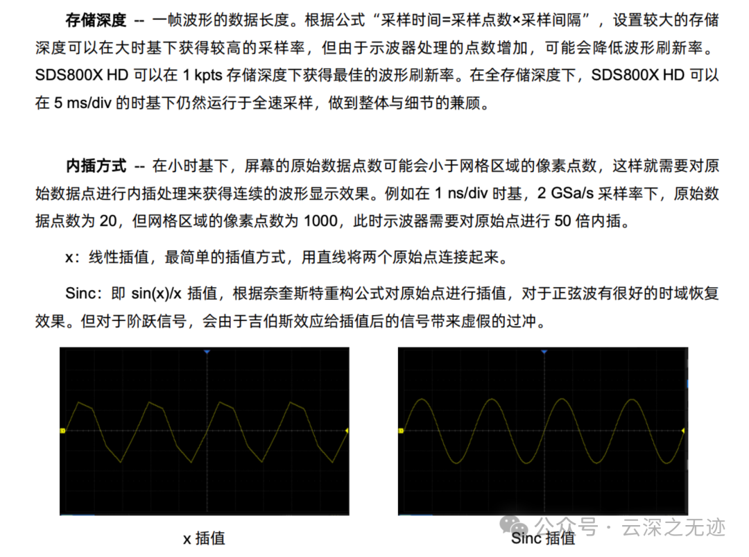
Linear Interpolation (x interpolation)
The simplest method is to connect two original points with a straight line. The advantage is fast computation, which can roughly show the trend; the disadvantage is that the curve looks angular and not realistic.
Sinc Interpolation (sin(x)/x interpolation)
Constructed based on the Nyquist sampling theorem, it serves as an ideal reconstruction filter; it can effectively restore the true waveform for continuous signals like sine waves.
The disadvantage is that for step signals, it introduces Gibbs phenomenon (ringing/overshoot at the edges).
Illustrative Comparison

Left image (x interpolation): The waveform appears angular, with noticeable distortion.
Right image (Sinc interpolation): The waveform is smooth, close to the true sine wave.
Let’s simulate and see the effect:
 Linear Interpolation and Sinc Interpolation comparison is very intuitive:
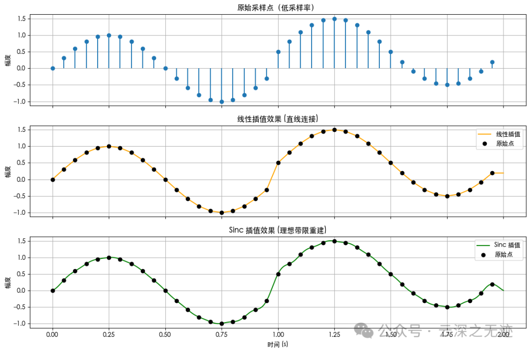
Top Image: Original Sample Points
The sampling rate is very low, and the points are sparse; the signal contains sine + step, so there are large gaps between points, making it look very discontinuous.
Middle Image: Linear Interpolation (x interpolation)
Directly connects two sample points with a straight line; the edges display realistically without false overshoot; however, the waveform looks like a polyline and is not smooth enough.
Bottom Image: Sinc Interpolation
Based on the ideal sampling reconstruction theorem, it can effectively restore the sine wave; the waveform is smooth and close to the true continuous signal; for step signals, ringing/overshoot occurs near the edges due to Gibbs phenomenon, which can be misleading.
Next, let’s look at the performance of a step signal:
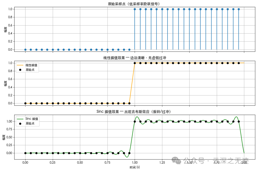
Top Image: Original Sample Points
The step points are very sparse, making it difficult to see clear edges directly.
Middle Image: Linear Interpolation
The edges are clear and crisp, directly pulling from 0 to 1; there is no false overshoot or ringing, making it suitable for observing digital signals and pulse signals.
Bottom Image: Sinc Interpolation
It can smoothly restore continuous signals, but at the step point, there is ringing/overshoot, which is the Gibbs phenomenon; although it looks “smoother”, the edges are not realistic and may mislead the user.
Next, let’s do a frequency response comparison (to see how much bandwidth of the signal linear interpolation and Sinc interpolation can restore), which can intuitively reflect the advantages of Sinc in the frequency domain:
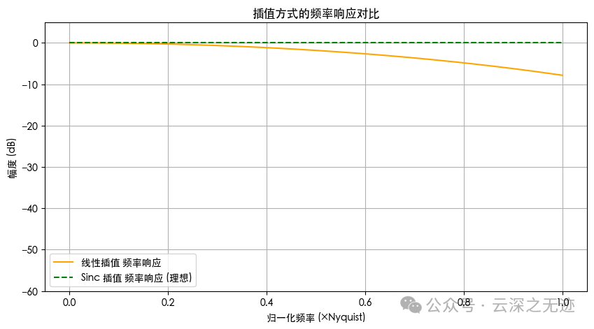
Linear Interpolation (orange curve)
Its frequency response is approximately that of a low-pass filter, with high-frequency components gradually attenuating; near Nyquist, the amplitude has already dropped by ~–8 dB.
This means: linear interpolation will lose high-frequency components, so the sine wave will appear “weakened” at high frequencies, and the edges will not be sharp enough.
Sinc Interpolation (green dashed line)
This is the ideal reconstruction filter, with a frequency response that remains flat (0 dB) across the entire 0~Nyquist range.
It can perfectly restore band-limited signals, so the sine wave appears very smooth on the screen; the downside is that for non-band-limited signals (like steps), it will introduce Gibbs phenomenon (false overshoot).
Linear Interpolation: Simple and fast, but essentially a low-pass filter that weakens high frequencies. Suitable for pulse/digital signals.
Sinc Interpolation: Ideal band-limited reconstruction that retains full bandwidth, but will have false overshoot at discontinuities. Suitable for sine/continuous signals.
Now let’s take a look at the display effects of high-frequency sine signals at low sampling rates with both types of interpolation:
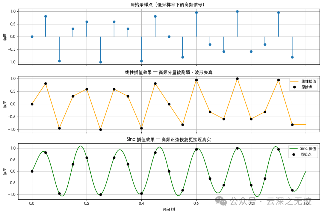
Top Image: Original Sample Points
The signal frequency is close to the Nyquist frequency (half of the sampling rate), and the points are very sparse; directly displaying it almost does not show a sine wave, just a bunch of discrete points.
Middle Image: Linear Interpolation
Points are connected with straight lines; high-frequency components are weakened, and the waveform is severely distorted, looking like a polyline; this indicates that linear interpolation will “low-pass” at high frequencies, resulting in inaccurate performance.
Bottom Image: Sinc Interpolation
It can restore a relatively smooth sine wave, close to the true signal; it retains the amplitude and shape of high-frequency components; this is the advantage of Sinc interpolation in the frequency domain.