MATLAB Code for Solving High-Order Partial Differential Equations Driven by PINNs

Reading time required:

6 minutes

Quick read only takes 2 minutes

Please respect the original work

Reprint must indicate the link to this article

and the author: Machine Learning Heart

Abstract: MATLAB code for solving high-order partial differential equations driven by PINNs.

Physics-Informed Neural Networks (PINNs) are a neural network method that combines deep learning with physical laws, aimed at solving problems involving partial differential equations (PDEs). Below is a detailed explanation of this problem:

1. Definition and Core Idea of Physics-Informed Neural Networks

Physics-Informed Neural Networks (PINNs) are a method that embeds physical laws into neural networks, guiding the training process of the neural network by using physical equations, boundary conditions, and initial conditions as constraints. This method can leverage known physical laws to enhance the model’s generalization ability, especially in cases of scarce or low-quality data.

2. Core Mechanism of PINNs

• Embedding of Physical Constraints: PINNs embed physical equations (such as partial differential equations) and boundary conditions into the loss function of the neural network, ensuring that the model automatically satisfies physical constraints during training. For example, the loss function typically includes terms for physical residuals and boundary condition residuals.
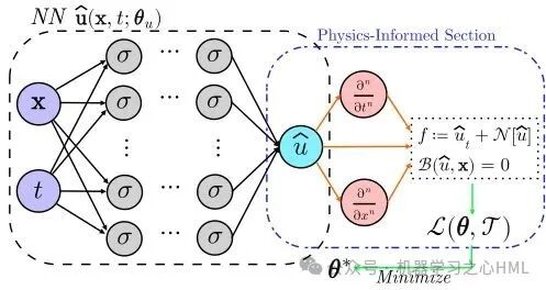
• Combination of Data-Driven and Physics-Driven Approaches: PINNs can utilize both data and physical knowledge for modeling, achieving good predictive results even with limited data.
• Flexibility and Scalability: PINNs can handle nonlinear problems, parameterized problems, and multiscale problems, and can address complex physical systems such as fluid dynamics, materials science, and geophysics.

3. Application Areas of PINNs

PINNs have been widely applied in various fields, including but not limited to:

• Fluid Mechanics and Fluid Dynamics: Used for simulating fluid flow, turbulence, wave propagation, etc.
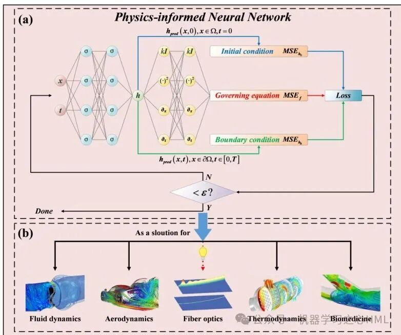
• Materials Science and Engineering: Used for simulating material behavior, microstructural mechanics, heterogeneous materials, etc.
• Biomedical and Medical Imaging: Used for image reconstruction, medical imaging, biological signal processing, etc.
• Energy and Environmental Science: Used for simulating energy systems, climate modeling, environmental dynamics, etc.

4. Advantages and Challenges of PINNs

• Advantages:

• High Data Efficiency: In cases of scarce data, PINNs can enhance the model’s generalization ability through physical constraints.
• Strong Interpretability: The introduction of physical constraints enhances the model’s interpretability, aiding in understanding the complex behavior of physical systems.
• High Computational Efficiency: Compared to traditional numerical methods (such as finite element methods), PINNs can have higher computational efficiency in certain cases.

• Challenges:

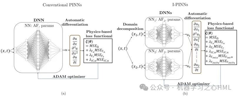
• Optimization Difficulty: The training process of PINNs can be complex, requiring careful tuning of hyperparameters (such as loss function weights, learning rates, etc.).
• Representation of Physical Equations: Accurately embedding complex physical equations and boundary conditions into the neural network remains a challenge.

5. Future Development Directions of PINNs

• Self-Adaptive Physics-Informed Neural Networks (SAPINNs): By introducing adaptive weights and dynamically adjusting physical constraints, further enhancing the model’s flexibility and adaptability.
• Multiscale and Multi-Physics Coupling: Developing PINNs models capable of handling multiscale and multi-physics coupling problems.
• Integration with Quantum Computing: Exploring the combination of PINNs with quantum computing to solve more complex physical problems.

Conclusion

Physics-Informed Neural Networks (PINNs) are an innovative method that combines deep learning with physical laws, effectively solving complex problems involving partial differential equations. By embedding physical constraints into the neural network, PINNs have significant advantages in cases of scarce data, low data quality, or complex physical systems. Despite challenges in optimization and representation of physical equations, PINNs show great application prospects in various fields.

2.1

The MATLAB code implements a high-order partial differential equation (beam vibration equation) solver based on Physics-Informed Neural Networks (PINN). Below is a detailed analysis:

1. Main Functions

main.m is the main program responsible for:

• Setting problem parameters (beam length L, time T, number of training points, etc.);
• Generating training data (PDE residual points, initial condition points, boundary condition points);
• Constructing the neural network structure;
• Training the neural network;
• Predicting solutions and visualizing results (comparing with analytical solutions, error analysis).

modelLoss.m is a custom loss function used for:

• Calculating PDE residuals, initial condition residuals, boundary condition residuals;
• Using automatic differentiation (dlgradient) to compute higher-order derivatives;
• Weighted combination of various losses and returning total loss and gradients.

2. Logical Connections

• main.m calls modelLoss.m to compute loss and gradients during training.
• modelLoss.m defines a loss function that includes constraints from physical equations (PDE), initial conditions (IC), and boundary conditions (BC), ensuring that the neural network learns physical laws.

3. Algorithm Steps

1. Data Generation: Randomly sample points in the spatial and temporal domains, including interior points, initial time points, and boundary points.
2. Network Construction: Construct a deep neural network using fully connected layers + tanh activation functions.
3. Training Loop:

• Using the Adam optimizer;
• Dynamically decaying learning rate;
• Calculating loss (PDE + IC + BC) and backpropagating each round.

4. Prediction and Evaluation:

• Predict solutions on the test grid;
• Compare with analytical solutions and calculate errors;
• Visualize results and training process.

4. Technical Route

• PINN Method: Embed the partial differential equation as a regularization term in the neural network loss function.
• Automatic Differentiation: Use dlgradient<code> to compute higher-order derivatives (e.g., ( u_{tt} ), ( u_{xxxx} )).
• Weighted Multi-Objective Loss: Assign higher weights to IC and BC to enhance constraints.
• Dynamically Decaying Learning Rate: Improve training stability.

5. Formula Principle

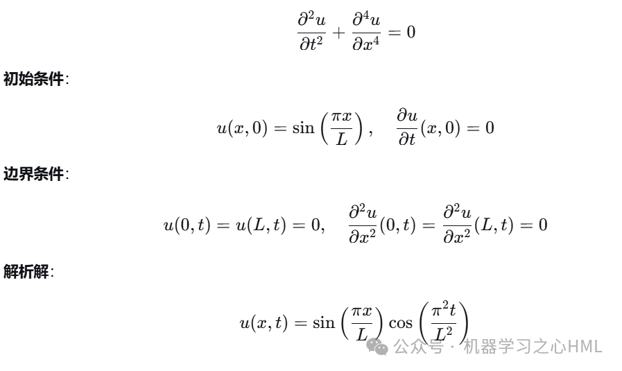
The equation being solved is the Euler-Bernoulli beam vibration equation:

6. Parameter Settings

Parameter	Meaning	Value
`<span>L</span>`	Beam length	1
`<span>T</span>`	Time length	1
`<span>numPDE</span>`	Number of PDE residual points	1000
`<span>numIC</span>`	Number of initial condition points	200
`<span>numBC</span>`	Number of boundary condition points	300
`<span>numEpochs</span>`	Number of training epochs	1000
`<span>initialLR</span>`	Initial learning rate	0.001
`<span>decayRate</span>`	Learning rate decay rate	0.95
`<span>decaySteps</span>`	Decay step length	100

7. Operating Environment

• Software: MATLAB2024b

Summary

This code uses the PINN method to solve the beam vibration equation, embedding physical constraints into the neural network training, avoiding the dependence on grids in traditional numerical methods, and is suitable for problems with complex boundary/initial conditions. The code structure is clear and includes a complete training, prediction, and visualization process, making it suitable as an introductory and practical case for PINNs.

2.2

Operating Results

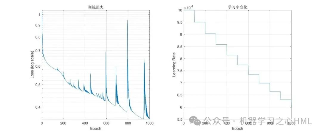
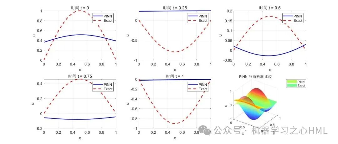
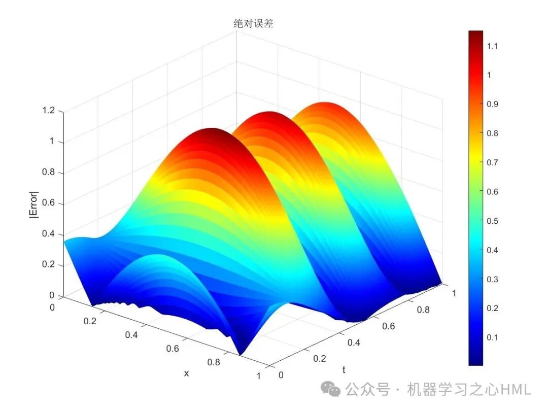
Complete code link:(It is recommended to copy the code link to a computer browser, use a certain F treasure to place an order, and click on the paid content to download the code directly):https://mbd.pub/o/bread/mbd-YZWXlZ9yZg==

Also can scan the QR code:

Partial Source Code

30px; } .lineNode {font-size: 10pt; font-family: Menlo, Monaco, Consolas, "Courier New", monospace; font-style: normal; font-weight: normal; }% Create a deeper neural networklayers = [    featureInputLayer(2, 'Name', 'input')   % Input layer (x,t)    fullyConnectedLayer(64, 'Name', 'fc1')  % Increase the number of neurons    tanhLayer('Name', 'tanh1')              % Activation function    fullyConnectedLayer(64, 'Name', 'fc2')    tanhLayer('Name', 'tanh2')    fullyConnectedLayer(64, 'Name', 'fc3')    tanhLayer('Name', 'tanh3')    fullyConnectedLayer(64, 'Name', 'fc4')  % Add extra layers    tanhLayer('Name', 'tanh4')    fullyConnectedLayer(64, 'Name', 'fc5')  % Add extra layers    tanhLayer('Name', 'tanh5')    fullyConnectedLayer(1, 'Name', 'output') % Output layer (u)];net = dlnetwork(layers);% Training parametersavgGrad = [];avgSqGrad = [];lossHistory = [];learningRates = [];% Create dlarray input datainputAll = dlarray([XAll, TAll]', "CB"); % 2×N matrix (x,t)

Other Codes

Well, the attentive you will find: https://mbd.pub/o/slowtrain/work

Blog Expert Certification, Creator in the field of Machine Learning, 2023 Blog Star TOP50, mainly engaged in programming and case analysis of machine learning and deep learning time series, regression, classification, clustering, and dimensionality reduction.Research project model customization/simulation of horizontal project models/guidance for academic papers on professional titles/model program explanation can contact me at QQ 1153460737 (Others are all pirated and scammers, please be careful)

Technical communication group: After purchasing any code from the blog or sharing the blog post to any third-party platform, you can add the author QQ to join the group

Machine Learning Heart OnlyQQ Number

Machine Learning Heart Only Channel Number

Previous Reviews:

Original unpublished! POD-PINN eigenvalue orthogonal decomposition combined with Physics-Informed Neural Network multivariable regression prediction model, MATLAB implementation

PINN Physics-Informed Neural Network used to solve boundary value problems of second-order ordinary differential equations (ODE), MATLAB implementation

Original! PINN Physics-Informed Neural Network univariate time series prediction, MATLAB implementation

PINN Physics-Informed Neural Network driven three-dimensional heat conduction equation solving MATLAB case

Exclusive original! PINN Physics-Informed Neural Network multivariable time series prediction, MATLAB implementation

Original first release! PINN Physics-Informed Neural Network multivariable regression prediction, MATLAB implementation