
The EKF example for three-dimensional state (strict derivation of combined navigation). Based on a 15-dimensional error state model: position (3), velocity (3), attitude (3), gyroscope bias (3), accelerometer bias (3). The observation is three-dimensional position (there is also a program for three-dimensional position + velocity as observations).
Article Directory
- Program Introduction
- Three-Dimensional EKF Combined Navigation System Code Structure Description
- Program Overview
- Code Structure Detailed Explanation
- Program Flow Overview
- Running Results
- MATLAB Source Code
Program Introduction
Three-Dimensional EKF Combined Navigation System Code Structure Description
Program Overview
This MATLAB program implements a three-dimensional combined navigation system based on the Extended Kalman Filter (EKF), integrating IMU (Inertial Measurement Unit) and GNSS (Global Navigation Satellite System) data to achieve high-precision position, velocity, and attitude estimation.
Code Structure Detailed Explanation
- Initialization Section (Lines 1-20)
% Basic settings
clear; clc; close all;
rng(0);% Fix random seed to ensure reproducibility
- Clear workspace and fix random seed
- Provide a reproducible simulation environment for the program
- System Parameter Configuration (Lines 21-35)
- Time Parameters: Sampling interval dt=0.1s, total simulation time 100s
- Noise Parameters: Define noise characteristics of IMU and GNSS
- Gyroscope noise, accelerometer noise
- Sensor bias parameters
- GNSS position observation noise
- Covariance Matrix Settings (Lines 36-50)
- Process Noise Matrix Q: 15×15 matrix describing system dynamic noise
- Observation Noise Matrix R: 3×3 matrix describing GNSS position observation noise
- Matrix is block-structured by state order: position, velocity, attitude, gyroscope bias, accelerometer bias
- State Vector and Data Storage Initialization (Lines 51-70)
- X_true: True trajectory state (15×N)
- X_imu: Pure IMU integration result (15×N)
- X_ekf: EKF filtering estimation result (15×N)
- Z: GNSS observation data (3×N)
- P: Initial covariance matrix
- Trajectory Generation and Sensor Data Simulation (Lines 71-105)
% Generate helical ascent motion trajectory
for k =1:N
% True trajectory calculation
% IMU data generation (acceleration and angular velocity)
% GNSS observation generation (updated every 1 second)
end
- Generate the true trajectory of helical ascent motion
- Simulate IMU sensor output (acceleration and angular velocity)
- Simulate GNSS observation data (position, 1Hz update rate)
- Pure IMU Integration Comparison Algorithm (Lines 106-125)
% Pure IMU integration as a comparison benchmark
for k =2:N
% Attitude update
% Velocity update
% Position update
% Bias random walk
end
- Implement pure IMU integration algorithm as a comparison benchmark
- Demonstrate the accumulation of IMU integration errors without filtering
- EKF Main Filtering Loop (Lines 126-160)
for k =2:N
% Prediction step
    X_pred =state_transition(X_ekf(:, k-1),imu_data(:, k-1), dt);
    F =compute_state_jacobian(X_ekf(:, k-1),imu_data(:, k-1), dt);
    P_pred = F * P * F'+ Q;

% Update step (when GNSS observation is available)
if~isnan(Z(1, k))
% Kalman gain calculation
% State and covariance update
end
end
Prediction step:
- Call state transition function for state prediction
- Calculate Jacobian matrix F
- Predict covariance matrix
Update step:
- Check GNSS observation availability
- Calculate Kalman gain
- Update state estimate and covariance
- Result Visualization (Lines 161-280)
Includes 5 main charts:
-
Three-Dimensional Trajectory Comparison Chart: Shows true trajectory, IMU integration, EKF estimation, and GNSS observation
-
Position Component Time Series Chart: Comparison of position in X, Y, Z directions
-
Velocity Component Time Series Chart: Comparison of velocity in X, Y, Z directions
-
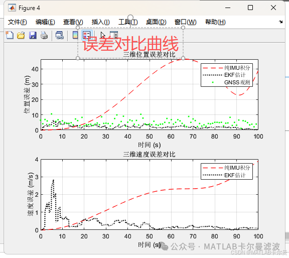
Position and Velocity Error Chart: Quantifies the accuracy of different methods
-
Attitude Angle Comparison Chart: Estimation effects of roll, pitch, and yaw angles
-
Performance Statistics Output (Lines 281-290)
-
Core Auxiliary Functions
Program Flow Overview
Initialization → Parameter Setting → Trajectory Generation → Pure IMU Integration → EKF Filtering → Result Visualization → Performance Analysis
Running Results
Three-Dimensional Trajectory Comparison Image: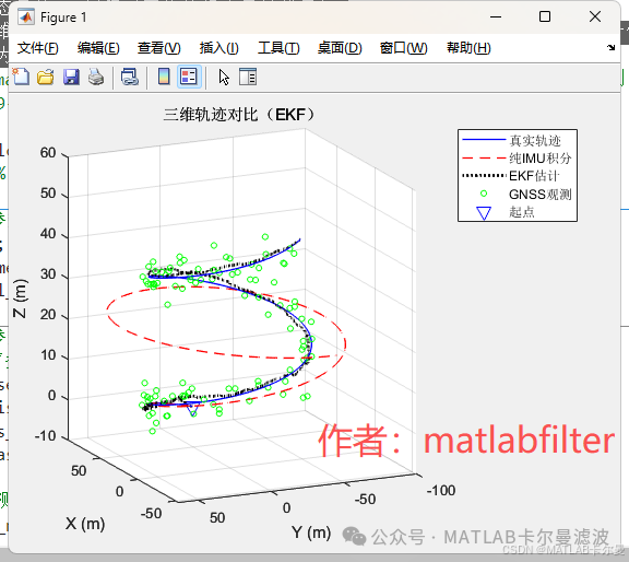 Velocity, Position, Attitude Comparison Chart: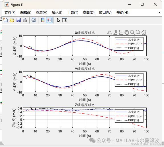
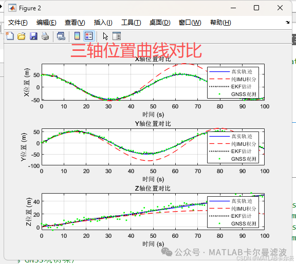
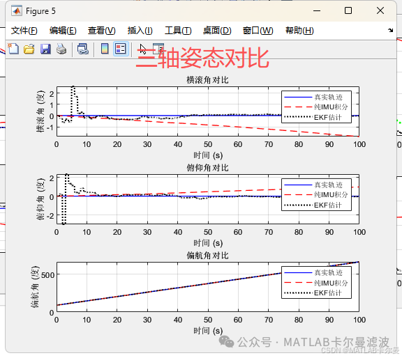 Error Comparison Image:
 Command Line Output Results: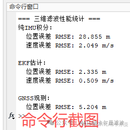
MATLAB Source Code
Partial code is as follows:
% EKF example for three-dimensional state (strict derivation of combined navigation)
% Based on a 15-dimensional error state model: position (3), velocity (3), attitude (3), gyroscope bias (3), accelerometer bias (3)
% The observation is three-dimensional position (there is also a program for three-dimensional position + velocity as observations on the shelf)
% Author: matlabfilter (WeChat same number), for custom MATLAB code related to positioning and navigation, filtering
% 2025-09-18/Ver1

clear; clc; close all;
rng(0);% Fix random seed

%% System Parameter Settings
dt =0.1;% Sampling time interval (s)
total_time =100;% Total simulation time (s)
N = total_time / dt;% Number of sampling points

%% Noise Parameter Settings
% IMU noise parameters
gyro_noise_std =0.01*pi/180;% Gyroscope noise standard deviation (rad/s)
accel_noise_std =0.001;% Accelerometer noise standard deviation (m/s^2)
gyro_bias_std =0.001*pi/180;% Gyroscope bias standard deviation (rad/s)
accel_bias_std =0.0001;% Accelerometer bias standard deviation (m/s^2)

% GNSS observation noise
gnss_pos_noise_std =3;% GNSS position noise standard deviation (m)
gnss_vel_noise_std =0.1;% GNSS velocity noise standard deviation (m/s)

%% Process Noise Covariance Matrix Q (15×15)
...
Full code:
https://mall.bilibili.com/neul-next/detailuniversal/detail.html?isMerchant=1&page=detailuniversal_detail&saleType=10&itemsId=13184342&loadingShow=1&noTitleBar=1&msource=merchant_share
Or click on “Read the original text” at the end to jump.
<span>If you need help or have custom code requirements related to navigation, positioning, and filtering, please contact the author via WeChat below</span>