Mobile Energy Pre-Layout and Dynamic Scheduling Strategies for Enhancing Resilience in Distribution Networks

Click the blue text above to follow us

📋📋📋 The table of contents is as follows: 🎁🎁🎁

Contents

💥1 Overview

📚2 Results

2.1 Pre-Disaster Prevention Phase

2.2 Post-Disaster Recovery Phase

🎉3 References

🌈4 Matlab Code, Data, Article Explanation

1 Overview

Source:

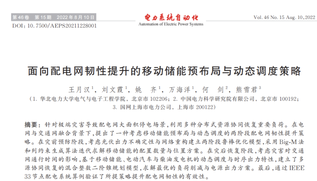
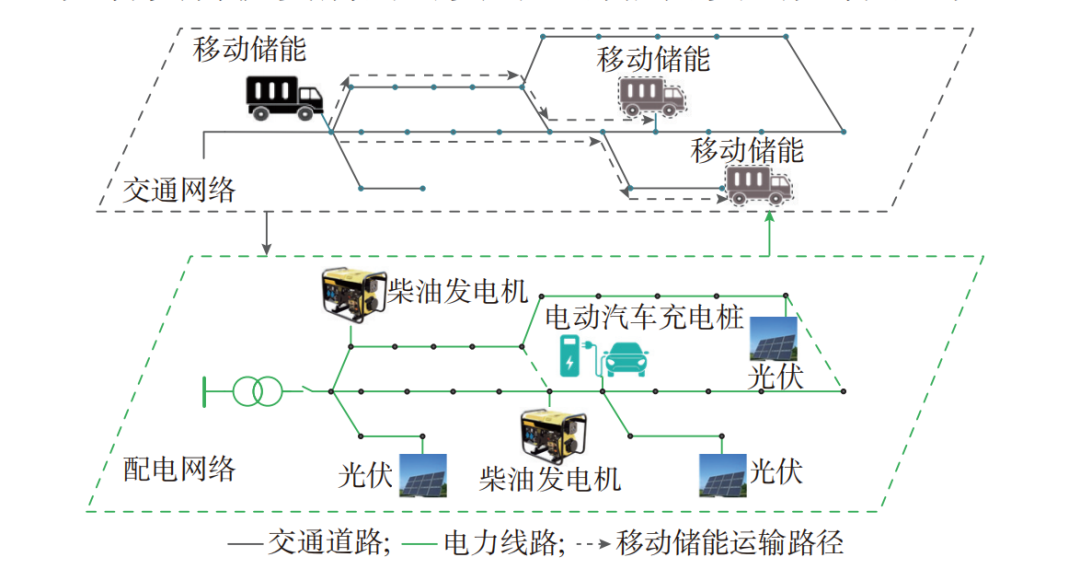
In recent years, extreme disasters have led to frequent large-scale power outages in the power grid. The resilience of the distribution network reflects the system’s ability to resist, adapt to, and recover from disasters, which has received widespread attention. Additionally, to address the dual crises of energy depletion and environmental pollution, a large number of distributed generation (DG) sources and electric load alternatives have been integrated into the distribution network, providing solutions for load recovery. Therefore, effectively utilizing various distributed resources before and after disasters to reduce power outage losses is of great significance for enhancing the resilience of the distribution network. Considering the integration of photovoltaic, mobile energy storage, electric vehicle charging stations (EVS), and diesel generators as distributed resources within the distribution network, the schematic structure of the grid-transportation network integration system is shown in Figure 1. Before a disaster, the load in the distribution network is powered by the upper-level main grid. After a disaster, the distribution network loses power from the main grid and experiences several line failures, affecting the real-time traffic capacity of the transportation network during the load recovery period. Currently, scholars both domestically and internationally have conducted extensive research on post-disaster recovery using distributed resources, mainly including island microgrids, emergency generators, and mobile resources. In the area of island microgrids, literature has proposed a microgrid formation mechanism that utilizes DG and remote control switches to restore important loads. Other studies have focused on restoring loads using diesel generators (DEG), fixed energy storage, and photovoltaic (PV) units when the main grid and distribution lines fail. Some have proposed load recovery methods based on planned microgrids to minimize load shedding costs when the main grid power supply is interrupted. Others have proposed recovery strategies considering load distribution and fuel-type DG site selection and sizing, which reduced the reserve capacity of emergency power sources. All of the above studies require pre-configured microgrids or a large number of fuel-type power sources, which have high investment costs and are not conducive to carbon reduction.

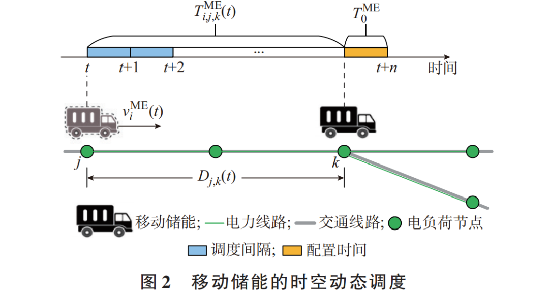
In the grid-transportation network integration system, the scheduling state of mobile energy storage is jointly determined by its charging and discharging state and transportation status, exhibiting spatiotemporal coupling characteristics. Considering the transportation time T_ME i,j,k (t) between nodes j and k for mobile energy storage i and the installation configuration time T0 ME, a spatiotemporal dynamic scheduling model for mobile energy storage is established, assuming that the transportation process does not consume electrical energy, as shown in Figure 2.

Research on Mobile Energy Storage Pre-Layout and Dynamic Scheduling Strategies for Enhancing Distribution Network Resilience

1. Definition and Evaluation Indicators of Distribution Network Resilience

1. Multistage Characteristics of Resilience The resilience of the distribution network is defined as the system’s ability to perform throughout the entire process during extreme events (such as natural disasters), including:

• Pre-Disaster: The ability to actively sense, predict disasters, and optimize resource layout (such as mobile energy storage).
• During Disaster: Robustness in resisting disturbances and maintaining power supply to critical loads.
• Post-Disaster: Adaptability and self-healing ability for rapid power restoration. Institutions such as the United States and the European Union have further refined resilience characteristics, such as robustness, agility, recovery, and learning ability.

Evaluation Indicators and Limitations

• Static Indicators: Based on network topology, connectivity, centrality, etc., reflecting the system’s structural resistance to destruction.
• Dynamic Indicators: Such as recovery time for power supply, load shedding costs, and the area under the system performance curve (resilience triangle/trapezoid model).
• Existing Issues: Existing indicators often focus on a single stage, lacking a dynamic multistage coupling evaluation system, and are insufficiently targeted towards disaster types (typhoons, earthquakes, etc.).

2. Basic Principles and Application Scenarios of Mobile Energy Storage Technology

1. Technical Principles

• Core Components: Battery packs (mainly lithium-ion), inverters, control systems, supporting flexible charging and discharging.
• Functional Characteristics: Plug-and-play, rapid response (millisecond level), movable deployment.
• Capacity Classification: Below 1 kWh for powering small devices, above 1 kWh for household backup or island operation.

Application Scenarios and Advantages

• Response to Extreme Events: Rapid recovery of power supply to critical loads post-disaster, replacing traditional fuel generators.
• Daily Optimization: Participation in peak shaving, voltage support, and reducing network losses.
• Limitations: Limited energy storage capacity, high costs (approximately 0.8-1.5 yuan/Wh), requiring collaborative optimization with distributed power sources.

3. Current Research Status of Mobile Energy Storage Pre-Layout Methods

1. Robust Optimization Model

• Two-Stage Model: Pre-disaster, optimizing the number and location of energy storage configurations based on the worst-case scenario (e.g., minimum photovoltaic output); post-disaster, minimizing losses through load shedding and network reconfiguration.
• Uncertainty Modeling: Using box-type uncertainty sets to describe fluctuations in photovoltaic output, combined with column constraint generation (C&CG) algorithms for solving.

Application of Intelligent Algorithms

• Particle Swarm Algorithm: Used for multi-objective optimization (e.g., minimizing network losses and voltage fluctuations).
• Genetic Algorithm: Solving nonlinear problems of energy storage site selection and sizing, improving convergence speed.

4. Typical Models of Dynamic Scheduling Strategies

1. Model Predictive Control (MPC)

• Rolling Optimization: Combining future state predictions with real-time feedback to achieve multi-time scale (hourly) scheduling.
• Application Scenarios: Optimizing energy storage charging and discharging and microgrid operation under fluctuations in wind and solar output.

Stochastic Optimization and Game Theory

• Scenario Analysis Method: Monte Carlo simulations generate extreme event scenario sets to assess expected load losses.
• Master-Slave Game: Coordinating electric vehicles (V2G mode) and mobile energy storage to achieve load transfer under price incentives.

5. Collaborative Strategies for Enhancing Distribution Network Resilience

1. Pre-Disaster and Post-Disaster Collaborative Optimization

• Pre-Layout Phase: Determining energy storage configurations through robust optimization to ensure rapid response post-disaster.
• Dynamic Scheduling Phase: Combining network reconfiguration, distributed generation (DG), and energy storage collaboration to maximize recovery of critical loads.

Multi-Energy System Coupling

• Electric-Gas-Heat Interconnection: Utilizing the redundancy of the natural gas network to enhance power supply resilience and reduce dependence on a single energy source.
• Transportation Network Collaboration: Scheduling electric vehicles as mobile energy storage units, optimizing charging station layouts and emergency power supply paths.

6. Case Studies of Collaborative Optimization

1. Two-Stage Robust Optimization Model (North China Electric Power University Case)

• Pre-Disaster Layout: Using C&CG algorithms to optimize energy storage configurations, reducing load shedding costs by 15%-20%.
• Post-Disaster Recovery: Through collaboration between mobile energy storage and DG, the recovery rate of critical loads increased to 78%.

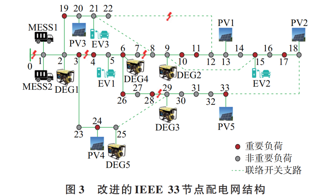
IEEE 33 Node Simulation Verification

• Result Comparison: After introducing mobile energy storage, the system resilience index (based on performance curve area) improved from 0.572 to 0.776.
• Economic Analysis: Configuration costs increased by 30%, but total operating costs (including load shedding losses) decreased by 45%.

7. Future Research Directions

1. Modeling for Multiple Disaster Types: Developing differentiated optimization models targeting different disaster characteristics such as typhoons and earthquakes.
2. Deep Integration of Renewable Energy: Researching the coupling mechanism of wind and solar output uncertainty with energy storage scheduling.
3. Standardized Indicator System: Establishing a dynamic multistage, multi-attribute decision-making resilience assessment framework.

Conclusion

Mobile energy storage, through collaborative optimization of pre-layout and dynamic scheduling, can significantly enhance the resilience of distribution networks during extreme events. Future efforts should further integrate multi-energy coupling and intelligent algorithms to build standardized assessment systems and promote the application of technology in practical engineering.

2 Results

2.1 Pre-Disaster Prevention Phase

Pre-disaster prevention uses the CCG algorithm, and the results obtained from running the following program are as follows:

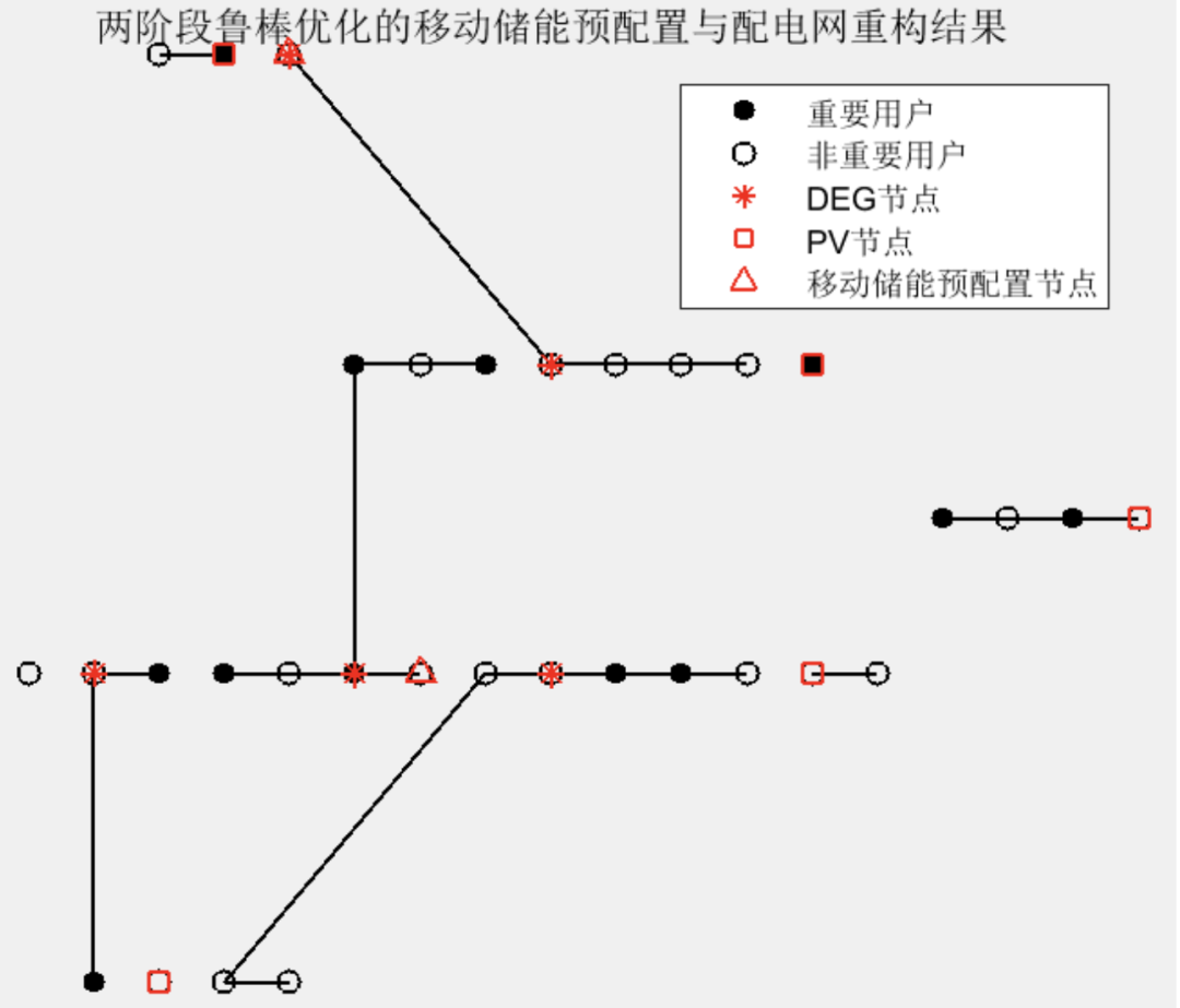
To better visualize the convergence of the CCG algorithm and the values of uncertain variables, two result graphs are provided.

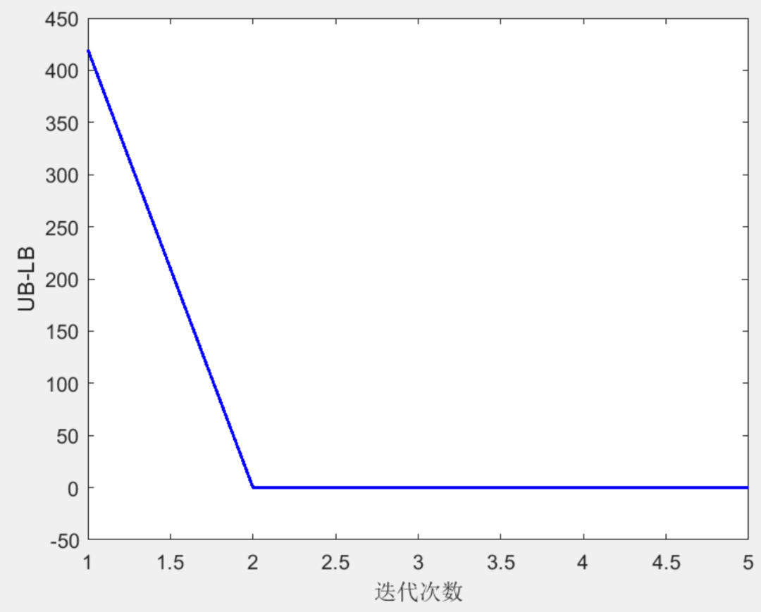
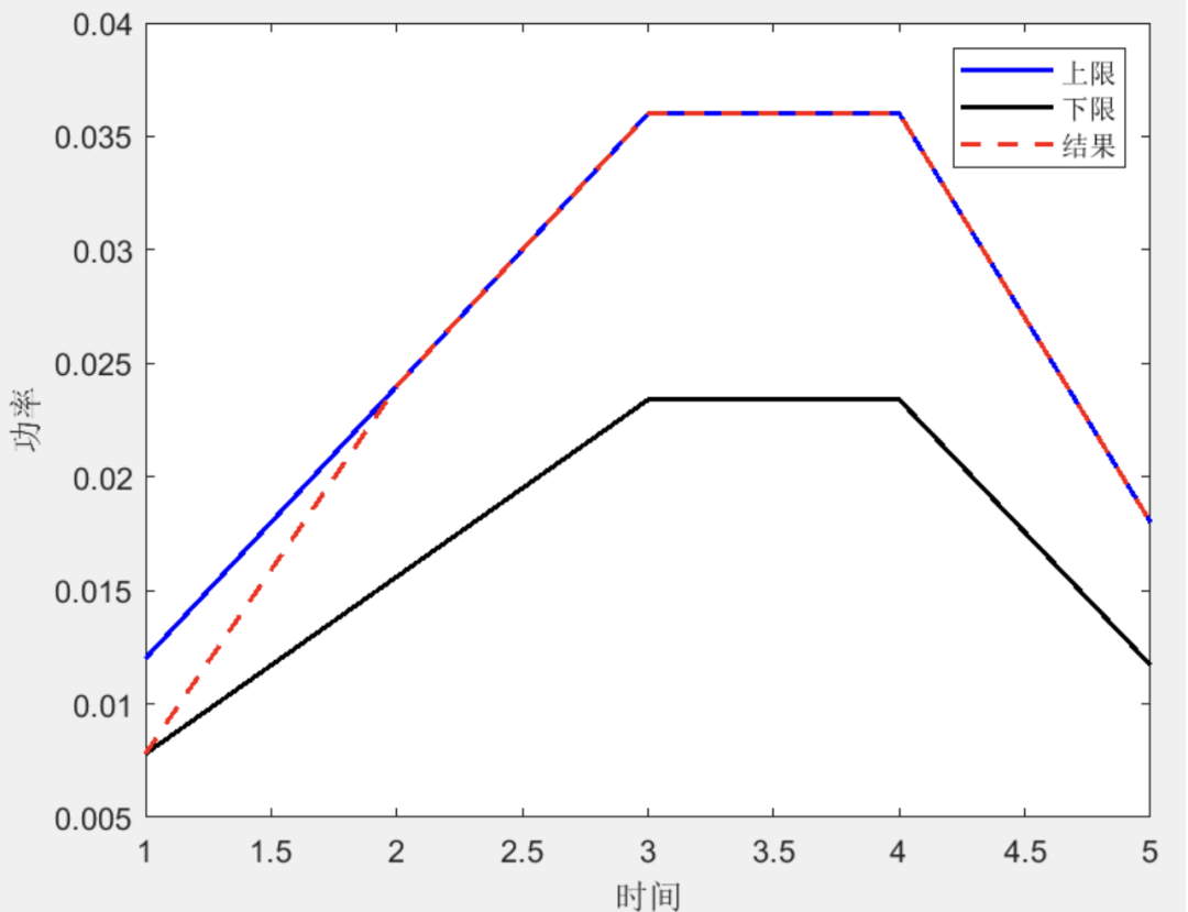
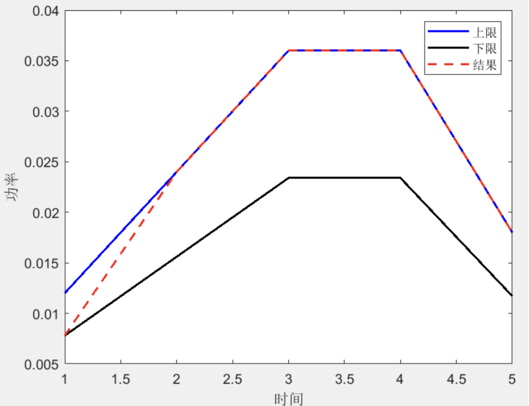
From the above two result graphs, it can be seen that the program converges completely after two iterations. The second graph shows the uncertainty distribution of photovoltaic output (considering only five time points). From the graph, it can be seen that except for the first time point, which is limited by the robustness conservativeness to the lower limit, all other time points are at the upper limit. The objective is to minimize energy storage configuration and load shedding costs, which contradicts common sense; as photovoltaic output decreases, costs should increase. To further verify the program issue, the photovoltaic output is set to the lower limit.

2.2 Post-Disaster Recovery Phase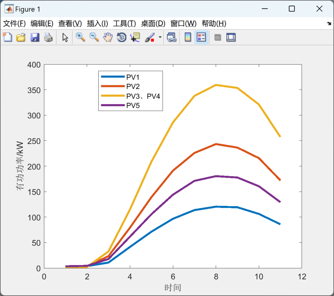

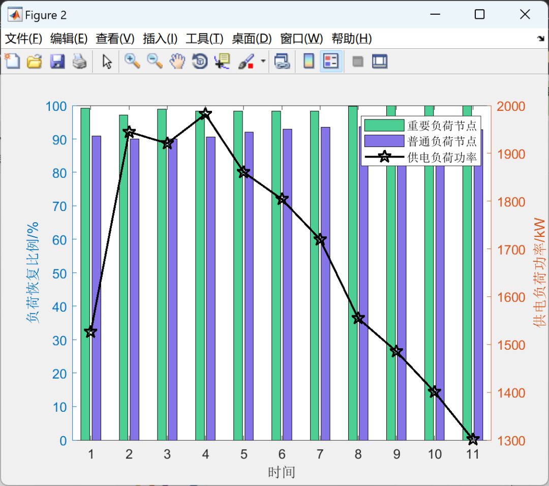
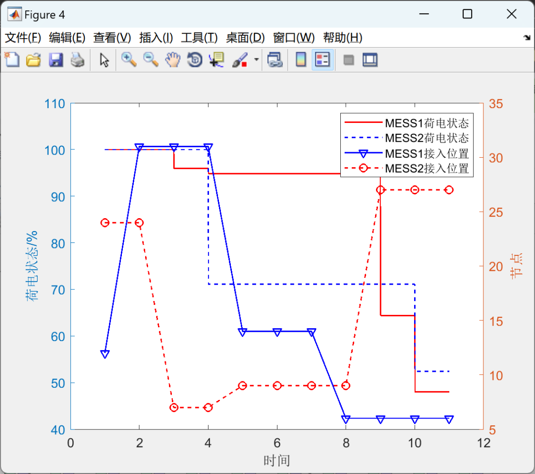
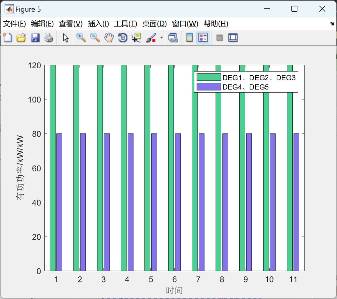
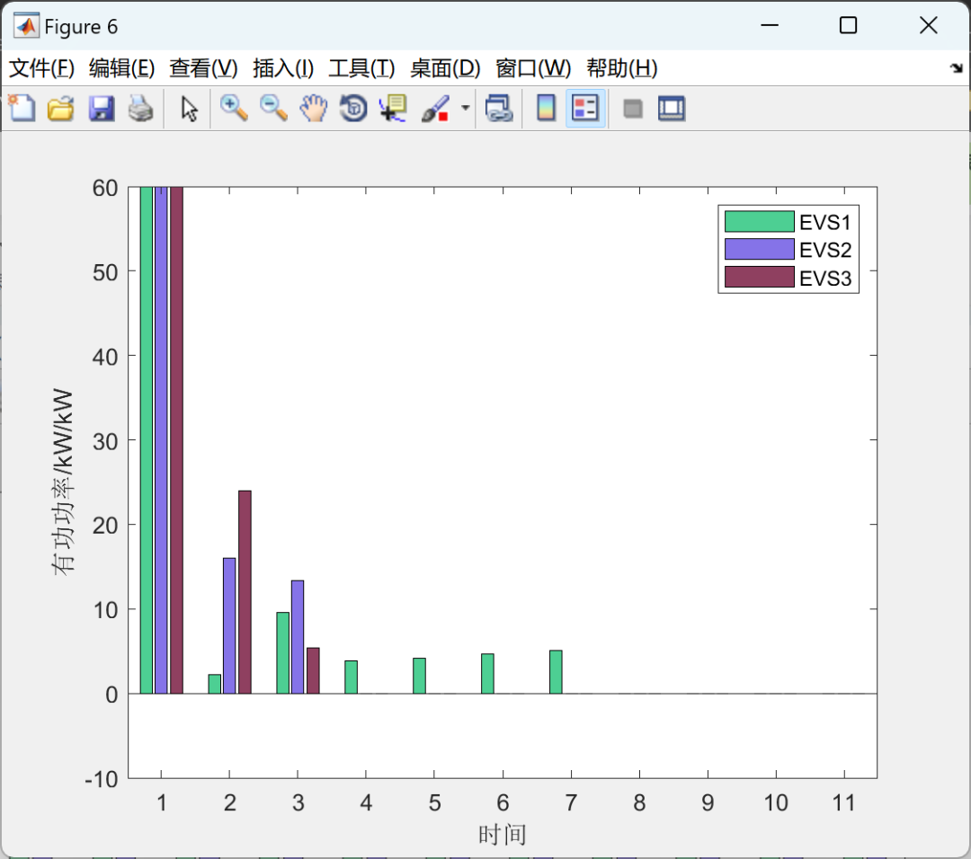
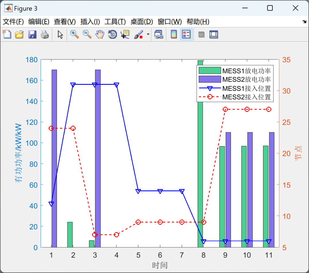
Partial code: clc close all %% Table 2 Dynamic scheduling results of mobile energy storage alpha_ME1 = value(alpha_ME1); alpha_ME2 = value(alpha_ME2); P_Mch = value(P_Mch); P_Mdch = value(P_Mdch); for t = 1:NT disp(['**************' , num2str(O_T(t)) , '：00时**************']) disp(['MESS1 connected node：' , num2str(find(alpha_ME1(:,t))) , '，charging and discharging power：' , num2str((P_Mdch(1,t) - P_Mch(1,t))*10000) , 'kW']) disp(['MESS2 connected node：' , num2str(find(alpha_ME2(:,t))) , '，charging and discharging power：' , num2str((P_Mdch(2,t) - P_Mch(2,t))*10000) , 'kW']) end %% Figure B3 Predicted output of photovoltaic units after disaster occurrence figure for k = 1:5 if k ~= 4 plot(pv_curve(:,k) , 'linewidth' , 2.5) hold on end end ylabel('Active Power/kW') xlabel('Time') legend('PV1','PV2','PV3','PV4','PV5') %% Figure 4 Load power and recovery ratio at each time period P_Lsu = value(P_Lsu); essential_load0 = sum(P_L_max(essential_user,:)); ordinary_load0 = sum(P_L_max(ordinary_user,:)); load0 = sum(P_L_max); essential_load1 = sum(P_L_max(essential_user,:) - P_Lsu(essential_user,:)); ordinary_load1 = sum(P_L_max(ordinary_user,:) - P_Lsu(ordinary_user,:)); load1 = sum(P_Lsu); figure yyaxis left e = bar([essential_load1./essential_load0*100; ordinary_load1./ordinary_load0*100]') color = [0.300956435005654, 0.810590442462569, 0.577780697646748; 0.521721248782275, 0.451274164510932, 0.911313227169849; 0.561880235062444, 0.249969169410276, 0.376220283460707; 0.241554770085929, 0.955437531793689, 0.228764772549632; 0.912720162652781, 0.142650346985794, 0.423524871222756; 0.825734269699093, 0.512563384780399, 0.273596220894793; 0.444545883918906, 0.971925137586938, 0.444565843866667; 0.982062563214574, 0.648320621265659, 0.627515046901424; 0.578267561462169, 0.614671003416509, 0.534641253536576; 0.234423496393930, 0.469650371915959, 0.385442159974304]; for i = 1:2 set(e(i),'FaceColor',color(i,:)); end ylabel('Load Recovery Ratio/%') hold on yyaxis right plot(load1*1000*SB , 'pentagramk-' , 'linewidth' , 1.5 , 'MarkerSize' , 10) ylabel('Power Supply Load/kW') legend('Critical Load Nodes','Ordinary Load Nodes','Power Supply Load') xlabel('Time') %% Figure B4 Relationship between active power output of mobile energy storage and connection location figure yyaxis left e = bar(P_Mdch'*10000) color = [0.300956435005654, 0.810590442462569, 0.577780697646748; 0.521721248782275, 0.451274164510932, 0.911313227169849; 0.561880235062444, 0.249969169410276, 0.376220283460707; 0.241554770085929, 0.955437531793689, 0.228764772549632; 0.912720162652781, 0.142650346985794, 0.423524871222756; 0.825734269699093, 0.512563384780399, 0.273596220894793; 0.444545883918906, 0.971925137586938, 0.444565843866667; 0.982062563214574, 0.648320621265659, 0.627515046901424; 0.578267561462169, 0.614671003416509, 0.534641253536576; 0.234423496393930, 0.469650371915959, 0.385442159974304]; for i = 1:2 set(e(i),'FaceColor',color(i,:)); end hold on ylabel('Active Power/kW/kW') yyaxis right ylabel('Node') for t = 1:NT MESS_node1(t) = find(alpha_ME1(:,t)); MESS_node2(t) = find(alpha_ME2(:,t)); end plot(MESS_node1 , 'bv-' , 'linewidth' , 1) plot(MESS_node2 , 'ro--' , 'linewidth' , 1) xlabel('Time') legend('MESS1 Discharge Power','MESS2 Discharge Power','MESS1 Connection Location','MESS2 Connection Location') %% Figure B5 Relationship between state of charge of mobile energy storage and connection location E_ME = value(E_ME); t0 = [12233445566778899101011]; E_ME0 = zeros(2,20); for t = 1:10 E_ME0(1,2*t-1) = E_ME(1,t); E_ME0(1,2*t) = E_ME(1,t); E_ME0(2,2*t-1) = E_ME(2,t); E_ME0(2,2*t) = E_ME(2,t); end figure yyaxis left plot(t1,E_ME0(1,:)*10000/6 , 'r' , 'linewidth' , 1) hold on plot(t1,E_ME0(2,:)*10000/6 , 'b' , 'linewidth' , 1) ylabel('State of Charge/%') yyaxis right ylabel('Node') for t = 1:NT MESS_node1(t) = find(alpha_ME1(:,t)); MESS_node2(t) = find(alpha_ME2(:,t)); end plot(MESS_node1 , 'bv-' , 'linewidth' , 1) plot(MESS_node2 , 'ro--' , 'linewidth' , 1) xlabel('Time') legend('MESS1 State of Charge','MESS2 State of Charge','MESS1 Connection Location','MESS2 Connection Location') %% Figure B6 Active power output of diesel generators during post-disaster recovery phase figure P_DG = value(P_DG); e = bar(P_DG([1,4],:)'*10000) color = [0.300956435005654, 0.810590442462569, 0.577780697646748; 0.521721248782275, 0.451274164510932, 0.911313227169849; 0.561880235062444, 0.249969169410276, 0.376220283460707; 0.241554770085929, 0.955437531793689, 0.228764772549632; 0.912720162652781, 0.142650346985794, 0.423524871222756; 0.825734269699093, 0.512563384780399, 0.273596220894793; 0.444545883918906, 0.971925137586938, 0.444565843866667; 0.982062563214574, 0.648320621265659, 0.627515046901424; 0.578267561462169, 0.614671003416509, 0.534641253536576; 0.234423496393930, 0.469650371915959, 0.385442159974304]; for i = 1:2 set(e(i),'FaceColor',color(i,:)); end ylabel('Active Power/kW/kW') xlabel('Time') legend('DEG1, DEG2, DEG3','DEG4, DEG5') %% Figure 5 Charging and discharging power of electric vehicle charging stations at each time period figure P_Ech = value(P_Ech); P_Edch = value(P_Edch); e = bar(P_Edch'*10000 - P_Ech'*10000) color = [0.300956435005654, 0.810590442462569, 0.577780697646748; 0.521721248782275, 0.451274164510932, 0.911313227169849; 0.561880235062444, 0.249969169410276, 0.376220283460707; 0.241554770085929, 0.955437531793689, 0.228764772549632; 0.912720162652781, 0.142650346985794, 0.423524871222756; 0.825734269699093, 0.512563384780399, 0.273596220894793; 0.444545883918906, 0.971925137586938, 0.444565843866667; 0.982062563214574, 0.648320621265659, 0.627515046901424; 0.578267561462169, 0.614671003416509, 0.534641253536576; 0.234423496393930, 0.469650371915959, 0.385442159974304]; for i = 1:3 set(e(i),'FaceColor',color(i,:)); end ylabel('Active Power/kW/kW') xlabel('Time') legend('EVS1','EVS2','EVS3')

References

Some theoretical sources are from the internet; if there is any infringement, please contact for removal.

[1] Wang Yuehan, Liu Wenxia, Yao Qi, et al. Research on Mobile Energy Storage Pre-Layout and Dynamic Scheduling Strategies for Enhancing Distribution Network Resilience. Automation of Electric Power Systems, 2022, 46(15): 37-45.

Matlab Code, Data, Article Explanation

Official AccountLychee Research Society