📡 Click the blue text above to follow ↑↑↑ 📡Research Background
In modern wireless communication systems, channel coding is a key technology to ensure the reliability of data transmission. In 2009, Arikan proposed Polar Codes, which is the first channel coding scheme strictly proven to achieve the Shannon limit under binary discrete memoryless channels, and has a relatively low encoding and decoding complexity. Therefore, it has been adopted as the coding method for control channels in 5G standards.
The core idea of Polar Codes is Channel Polarization, which transforms the original channel into two types of sub-channels—reliable channels and unreliable channels—through the joint and split of channels. Information bits are mapped to reliable channels, while unreliable channels are fixed as Frozen Bits. The encoding process can be completed using a generator matrix, and for a given code length, its generator matrix is:
Where denotes the thKronecker product, the base matrix and Kronecker product are defined as:
And is the th identity matrix, is a bit-flipping matrix, and represents a permutation operation that places odd positions in front and even positions behind. The encoding process can be expressed as:, where is the input bit sequence, frozen bits are fixed to 0, and information bits are mapped to reliable channels, ultimately obtaining the codeword . The complexity of this process is , making it efficient for hardware implementation. To ensure the correct information is received, an efficient decoding algorithm is also required. Common decoding methods for Polar Codes mainly fall into two categories:
- Successive Cancellation (SC/SCL) Decoding: Simple to implement but has high latency and poor performance for short code lengths.
- Belief Propagation (BP) Decoding: Based on factor graph iteration, it has strong parallelism and low latency, making it more suitable for hardware implementation, but it has high computational complexity.
In recent years, researchers have made many optimizations to BP decoding, such as:
- Introducing Early Stopping Mechanism to reduce the number of iterations;
- Using Min-Sum Approximation to reduce computational complexity;
- Combining Deep Learning with BP Algorithm, mapping the factor graph to a neural network, and introducing trainable scaling factors, significantly improving convergence speed and decoding performance. Based on this, this paper introduces the BP decoding algorithm combined with neural networks and implements it on FPGA for simulation testing.
System Model Overall Structure
Belief Propagation (BP) Decoding Algorithm for Polar Codes is an iterative method based on factor graphs. Its basic idea is:
- To pass Log-Likelihood Ratio (LLR) messages between nodes in the factor graph, continuously updating belief values;
- In each iteration, first pass L messages (from right to left), then pass R messages (from left to right), with nodes updating progressively;
- After multiple iterations, use the final LLR values to decide the bits, thus obtaining the decoding results.
Compared to serial decoding, BP has strong parallelism and lower latency, making it more suitable for hardware implementation. For traditional BP decoding algorithms, taking Polar Codes of length as an example, its corresponding factor graph contains layers, with computation units per layer.
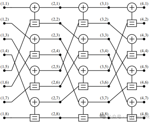
In this factor graph, each computation unit receives two inputs and outputs two results, structured as shown in the figure, with nodes responsible for continuously passing and updating LLR (Log-Likelihood Ratio) messages.
The core computation formula is:
Where the exact form of the function is:
, due to its high computational complexity, the Min-Sum Approximation is usually used for simplification in hardware implementations:. At the beginning of the iteration, the confidence of the nodes corresponding to the frozen bits is initialized to infinity, indicating that these bits are fixed. After multiple iterations, the final LLR values are used for hard decision-making to obtain the decoding results,Decision Rule is:
Traditional BP decoding algorithms usually require many iterations (e.g., 20-30 times) to achieve low error rates in decoding results. Multiple iterations increase the overall decoding time, resulting in more latency and requiring storage of a large number of intermediate LLR messages,leading to high resource overhead. Therefore, neural networks are introduced into BP decoding to optimize iteration efficiency and improve decoding performance, with the main idea being:
- Mapping the factor graph of Polar Codes to a neural network structure, with each iteration corresponding to a layer in the network;
- Introducing trainable scaling factors in the Min-Sum Approximation, allowing the neural network to learn optimal parameters;
The new iteration update formula is:
Where and are scaling factors, optimized and updated through training, allowing for better error performance than traditional BP with fewer iterations.
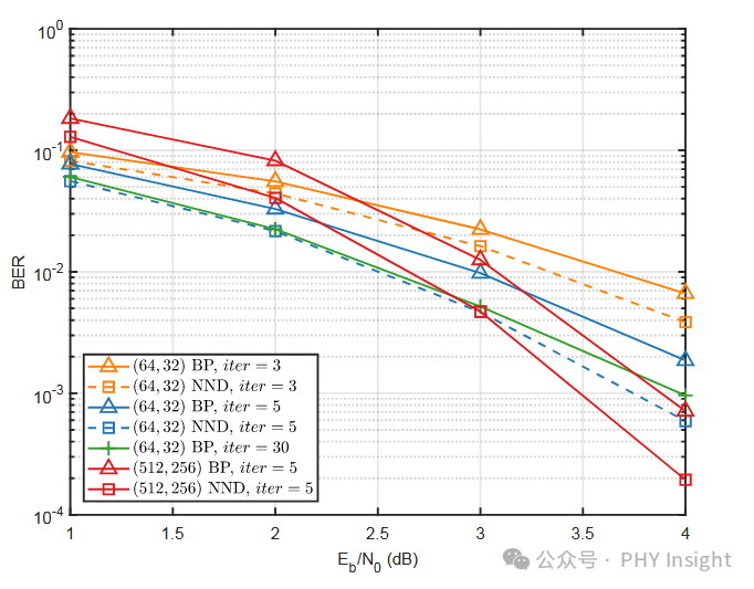
For the (64, 32) Polar Code, NND can achieve the effect of traditional BP after 30 iterations in just 5 iterations. Therefore, the neural network combined BP decoding reduces the number of iterations and latency, and its parallel structure is also suitable for implementation on hardware platforms such as FPGA.
Hardware Implementation and Simulation Testing
Based on the neural network combined BP decoding algorithm, implementation is carried out on the FPGA platform, using trained scaling parameters, mainly to realize the decoding inference process. On the hardware side, a parallel structure is adopted to improve throughput, using INT8 Quantization to compress bit width, reducing resource consumption while ensuring performance. The overall architecture follows the process of “Input Preprocessing → Confidence Propagation (Left and Right Iteration) → Result Decision”.The entire training process of the decoder is completed in the Tensorflow Framework, in the BP decoder part, first initializing based on channel output and frozen bit positions, then iteratively updating according to the formula, and after multiple iterations, making decisions based on the final LLR values:
LV = tf.Variable(np.float32(np.ones((n, N, bp_iter_num))))RV = tf.Variable(np.float32(np.ones((n, N, bp_iter_num))))def bp_algorithm(bp_iter_num, net_dict, FZlookup, batch_size, bp1_input): bp_input = tf.matmul(bp1_input, one_matre) for i in range(n + 1): for j in range(N): net_dict["L_{0}{1}{2}".format(i, j, 0)] = tf.zeros((batch_size)) net_dict["R_{0}{1}{2}".format(i, j, 0)] = tf.zeros((batch_size)) for j in range(N): net_dict["L_{0}{1}{2}".format(n, j, 0)] = tf.ones((1)) * bp_input[:, j] if FZlookup[j] == 0: net_dict["R_{0}{1}{2}".format(0, j, 0)] = tf.ones((batch_size)) * inf_num # bp algorithm for j in range(bp_iter_num): itr = j for i in range(n, 0, -1): for phi in range(2**i): psi = int(np.floor(phi / 2)) if np.mod(phi, 2) != 0: for omega in range(2 ** (n - i)): net_dict["R_{0}{1}{2}".format(n + 1 - i, psi + 2 * omega * 2 ** (i - 1), 0)] = RV[n - i, psi + 2 * omega * 2 ** (i - 1), itr] * fFunction(net_dict["L_{0}{1}{2}".format(n + 1 - i, psi + (2 * omega + 1) * 2 ** (i - 1), 0)] + net_dict["R_{0}{1}{2}".format(n - i, psi + (2 * omega + 1) * 2 ** (i - 1), 0)], net_dict["R_{0}{1}{2}".format(n - i, psi + 2 * omega * 2 ** (i - 1), 0)]) net_dict["R_{0}{1}{2}".format(n + 1 - i, psi + (2 * omega + 1) * 2 ** (i - 1), 0)] = net_dict["R_{0}{1}{2}".format(n - i, psi + (2 * omega + 1) * 2 ** (i - 1), 0)] + RV[n - i, psi + (2 * omega + 1) * 2 ** (i - 1), itr] * fFunction(net_dict["L_{0}{1}{2}".format(n + 1 - i, psi + 2 * omega * 2 ** (i - 1), 0)], net_dict["R_{0}{1}{2}".format(n - i, psi + 2 * omega * 2 ** (i - 1), 0)]) for i in range(1, n + 1): for phi in range(2**i): psi = int(np.floor(phi / 2)) if np.mod(phi, 2) != 0: for omega in range(2 ** (n - i)): net_dict["L_{0}{1}{2}".format(n - i, psi + 2 * omega * 2 ** (i - 1), 0)] = LV[n - i, psi + 2 * omega * 2 ** (i - 1), itr] * fFunction(net_dict["L_{0}{1}{2}".format(n + 1 - i, psi + 2 * omega * 2 ** (i - 1), 0)], net_dict["L_{0}{1}{2}".format(n + 1 - i, psi + (2 * omega + 1) * 2 ** (i - 1), 0)] + net_dict["R_{0}{1}{2}".format(n - i, psi + (2 * omega + 1) * 2 ** (i - 1), 0)]) net_dict["L_{0}{1}{2}".format(n - i, psi + (2 * omega + 1) * 2 ** (i - 1), 0)] = net_dict["L_{0}{1}{2}".format(n + 1 - i, psi + (2 * omega + 1) * 2 ** (i - 1), 0)] + LV[n - i, psi + (2 * omega + 1) * 2 ** (i - 1), itr] * fFunction(net_dict["L_{0}{1}{2}".format(n + 1 - i, psi + 2 * omega * 2 ** (i - 1), 0)], net_dict["R_{0}{1}{2}".format(n - i, psi + 2 * omega * 2 ** (i - 1), 0)]) llr_output = tf.zeros((1)) for i in range(N): if FZlookup[i] == -1: llr_output = tf.concat([llr_output, net_dict["L_{0}{1}{2}".format(0, i, 0)]], 0) llr_output = tf.transpose(tf.reshape(llr_output[1:], (K, batch_size))) * -1 return llr_outputWhen implementing the decoder on FPGA, a large amount of LLR data needs to be stored, and floating-point operations (such as FP32) consume many logic units, DSP resources, and registers. Therefore, data compression is necessary to improve computational efficiency and reduce resource consumption. The quantization methods mainly include:
| Quantization Scheme | Bit Width | Description | FPGA Compatibility |
|---|---|---|---|
| FP32 | 32 | Default training format, highest precision, extremely high resource overhead | ❌ Not recommended |
| FP16 | 16 | Common half-precision inference for GPUs, requires additional floating-point multiply-add units | ⚠️ Some FPGA support |
| INT8 | 8 | Mainstream deployment scheme, good balance between performance and precision | ✅ Efficient mapping |
| INT4 | 4 | Extreme compression scheme, suitable for distilled models | ✅ Requires Lookup optimization |
| Mixed-Precision | Variable | Different layers use different bit widths | ✅ High compilation cost |
In practical engineering, INT8 symmetric quantization is usually used to fully leverage FPGA’s advantages in fixed-point operations. Additionally, since the BP decoding algorithm requires initializing the confidence of the frozen bits to infinity, this affects the quantization calibration process. Therefore, within the quantization range of INT8, special handling of extreme values is needed to represent positive and negative infinity separately.
The trained scaling parameters are imported into the FPGA for testing after quantization calibration. The entire decoding process follows the order of “Confidence Initialization → Left Propagation → Right Propagation → Hard Decision”, utilizing the parallel characteristics of FPGA to complete the confidence calculation and updating of the entire layer within one clock cycle, ensuring the efficient execution of the decoding process.
Taking the (64,32) Polar Code as an example, its corresponding decoding network layer number is n=\log_{2}{N}=6, and testing is conducted under the iteration number iterNum=3, with the testing environment frequency CLK=100MHz, the received input data are 32’b01000100010000101110101111111100, 32’b11101000001111101101010110000000, 32’b01101111010111010101001011111111, and the corresponding test results are as follows:

Where out represents the decoding result, which matches the input data exactly. Since each iteration includes one left propagation and one right propagation, the total clock cycle count is Count=IterNum*n*2, achieving a significant reduction in latency compared to traditional BP decoders.
Core Code
Below is a sample of the core code, where the quantization parameters are approximated using power scaling for easier hardware implementation:.
Basic Computing Unit
module BCB #( parameter width = 8, parameter fix_width = 24) (a, b, c, d,a_int, a_exp, b_int, b_exp,c_int, c_exp, d_int, d_exp,res_int,res_exp,result); input signed [width-1:0] a, b, c, d; input signed [31:0] a_int, a_exp, b_int, b_exp, c_int, c_exp, d_int, d_exp, res_int, res_exp; output signed [width-1:0] result; wire signed [fix_width-1:0] dq_a, dq_b, dq_c, dq_d; wire signed [fix_width-1:0] sum_ab; wire signed [fix_width-1:0] func_out; wire signed [fix_width-1:0] mul_out; dequant #(.fix_width(fix_width)) dq_mod_a (.quantized(a), .b(a_int), .c(a_exp), .result(dq_a)); dequant #(.fix_width(fix_width)) dq_mod_b (.quantized(b), .b(b_int), .c(b_exp), .result(dq_b)); dequant #(.fix_width(fix_width)) dq_mod_c (.quantized(c), .b(c_int), .c(c_exp), .result(dq_c)); dequant #(.fix_width(fix_width)) dq_mod_d (.quantized(d), .b(d_int), .c(d_exp), .result(dq_d)); adder_2in #(.WIDTH(fix_width)) adder_ab (.i_a(dq_a), .i_b(dq_b), .o(sum_ab)); fFunct #(.width(fix_width)) f_func (.a(dq_c), .b(sum_ab), .out(func_out)); mult_2in #(.WIDTH(fix_width)) mult_inst (.i_a(func_out), .i_b(dq_d), .o(mul_out)); quant #(.fix_width(fix_width))quantizer(.data(mul_out),.b(res_int),.c(res_exp), .quantized(result));endmoduleOther Submodules:
In the dequantization part, the INT8 data is restored to fixed-point numbers in 12.12 format based on the input data and quantization parameters;
// Dequantization module dequant #(parameter fix_width = 24) ( input signed [7:0] quantized, input signed [31:0] b, input signed [31:0] c, output reg signed [fix_width-1:0] result ); reg signed [39:0] product; reg signed [63:0] shifted; integer total_shift; always @(*) begin if (quantized == 8'sd127) begin result = 24'sh3E8000; end else if (quantized == -8'sd127) begin result = -24'sh3E8000; end else begin product = quantized * b; total_shift = c + 12; shifted = {{24{product[39]}}, product}; if (total_shift >= 0) begin shifted = shifted << total_shift; end else begin shifted = shifted >>> (-total_shift); end result = shifted[23:0]; end endendmoduleIn the quantization part, the input data is compressed into INT8 integer representation using quantization parameters.
// Quantization module quant #(parameter fix_width = 24) ( input signed [23:0] data, input signed [31:0] b, input signed [31:0] c, output reg signed [ 7:0] quantized ); integer total_shift; reg signed [63:0] scale; reg signed [63:0] scaled_data; reg signed [63:0] rounded_data; reg special_case; localparam signed [23:0] THRESHOLD = 24'd1000 << 12; localparam signed [23:0] RANGE = 24'd10 << 12; localparam integer FRAC_BITS = 12; always @(*) begin // Extreme value handling special_case = ((data > (THRESHOLD - RANGE)) && (data < (THRESHOLD + RANGE))) ||((data > -(THRESHOLD + RANGE)) && (data < -(THRESHOLD - RANGE))); if (special_case) begin if (data >= 0) begin quantized = 8'sd127; end else begin quantized = -8'sd127; end end else begin total_shift = c + 12; scale = {{32{b[31]}}, b}; if (total_shift >= 0) begin scale = scale << total_shift; end else begin scale = scale >>> (-total_shift); end scaled_data = (data << FRAC_BITS) / scale; // Round the result rounded_data = scaled_data + (1 << (FRAC_BITS - 1)); // Control within INT8 range if (rounded_data < (-126 << FRAC_BITS)) begin quantized = -8'sd126; end else if (rounded_data > (126 << FRAC_BITS)) begin quantized = 8'sd126; end else begin // Convert back to integer by right shifting quantized = rounded_data >>> FRAC_BITS; end end endendmodulefFunct module receives two inputs and outputs their Min-Sum approximation result.
// Min-Sum Approximation Function module fFunct #(parameter width = 24) (a,b,out); input signed [width-1:0] a; input signed [width-1:0] b; output signed [width-1:0] out; wire signed [width-1:0] sign_a; wire signed [width-1:0] sign_b; wire signed [width-1:0] abs_a; wire signed [width-1:0] abs_b; wire signed [width-1:0] min_val; wire signed [width-1:0] res; assign sign_a = (a < 0) ? -1 : 1; assign sign_b = (b < 0) ? -1 : 1; assign abs_a = (a < 0) ? -a : a; assign abs_b = (b < 0) ? -b : b; assign min_val = (abs_a < abs_b) ? abs_a : abs_b; assign res = sign_a * sign_b * min_val; assign out = res;endmodulePaper Information
L. Xiang, J. Cui, J. Hu, K. Yang and L. Hanzo, “Polar Coded Integrated Data and Energy Networking: A Deep Neural Network Assisted End-to-End Design,” in IEEE Transactions on Vehicular Technology, vol. 72, no. 8, pp. 11047-11052, Aug. 2023, doi: 10.1109/TVT.2023.3262624.
Click below to read the original text download the paper
Authors: Kui Lv, Jingwen Cui, Leping Xiang
Editor: Cheng Luo