Data Decomposition Method Based on MATLAB Language VMD Variational Mode Decomposition1. VMD addresses the shortcomings of traditional EMD theory, such as endpoint effects and mode mixing, and can be used for various problems including signal decomposition, original signal graphs, decomposition effect graphs, and spectrum graphs.

The following text and example code are for reference only.

Table of Contents

• Detailed Explanation and Implementation of VMD (Variational Mode Decomposition) Data Decomposition Method Based on MATLAB
• 1. Introduction to VMD Method
• Core Idea:
• 2. MATLAB Implementation Steps
• 1. Install VMD Toolbox
• 3. VMD MATLAB Example Code
• Example: VMD Decomposition of Synthetic Signal
• 4. Core Function `VMD.m` (can be saved separately)
• 5. Parameter Description
• 6. Application Areas
• 7. Conclusion

Detailed Explanation and Implementation of VMD (Variational Mode Decomposition) Data Decomposition Method Based on MATLAB

1. Introduction to VMD Method

VMD (Variational Mode Decomposition) is a novel signal adaptive decomposition method that can decompose complex multi-component signals into several intrinsic mode functions (IMFs) with specific center frequencies and bandwidths. Compared to traditional methods like EMD and EEMD, VMD has better noise resistance and mathematical theoretical support.

Core Idea:

• Decomposing the original signal into multiple mode functions (referred to as IMF or mode components)
• Each mode function is compact in the time domain and has a clear center frequency in the frequency domain
• The decomposition process is completed by constructing and solving a constrained variational problem

2. MATLAB Implementation Steps

1. Install VMD Toolbox

VMD is not integrated into the official MATLAB toolbox and needs to be downloaded manually:

GitHub Address: https://github.com/zhaoshensi/Variational-Mode-Decomposition

Or directly use the following code snippet (simplified version).

3. VMD MATLAB Example Code

Example: VMD Decomposition of Synthetic Signal

% MATLAB VMD Variational Mode Decomposition Example

clear; clc; close all;

%% 1. Construct Synthetic Signal
fs =1000;% Sampling rate
T =1;% Time length 1s
t =(0:1/fs:T-1/fs)';% Time vector

% Construct a multi-component signal
f1 =5; f2 =10; f3 =20; f4 =40;
signal =sin(2*pi*f1*t).*(t <=0.5)+...
sin(2*pi*f2*t).*(t >0.5 && t <=1.0)+...
0.5*cos(2*pi*f3*t)+...
0.2*sin(2*pi*f4*t);

% Add Gaussian white noise
signal = signal +0.2*randn(size(t));

%% 2. Set VMD Parameters
alpha =2000;% Penalty factor (the larger, the stricter the reconstruction)
tau =0;% Noise tolerance, generally set to 0 (in the absence of noise)
K =4;% Number of decomposition modes
DC =0;% Whether there is a DC component (0 means none)
init =1;% Initialization method (1: uniform distribution; 2: random)
tol =1e-7;% Convergence tolerance

%% 3. Call VMD Function
[imf, u_hat, omega]=VMD(signal, alpha, tau, K, DC, init, tol);

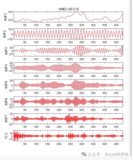
%% 4. Plot Results
figure;
subplot(K+1,1,1);
plot(t, signal,'k');
title('Original Signal');

for k =1:K
subplot(K+1,1, k+1);
plot(t,imf(:,k));
title(['IMF ',num2str(k)]);
end

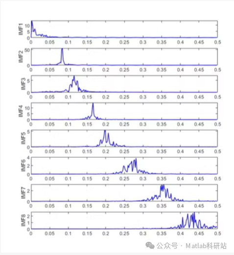
%% 5. Visualize Spectrum
figure;
for k =1:K
subplot(K,1, k);
[Pxx,F]=pwelch(imf(:,k),[],[],[], fs);
plot(F,10*log10(Pxx));
xlim([0 fs/2]);
ylabel('PSD (dB)');
title(['IMF ',num2str(k),' Spectrum']);
end

4. Core Function <span>VMD.m</span> (can be saved separately)

The following is a simplified version of the <span>VMD.m</span> function, which can be saved as a file with the same name to run.

function[u, u_hat, omega]=VMD(signal, alpha, tau, K, DC, init, tol)
% References:
% Dragomiretskiy, K. and Zosso, D. (2014) Variational Mode Decomposition
% IEEE Trans. on Signal Processing, vol. 62, no. 3

% Input parameter description:
% signal - Original input signal
% alpha - Penalty factor
% tau - Noise tolerance
% K - Number of decomposition modes
% DC - Whether to include DC component (0/1)
% init - Initialization method (1: uniform distribution; 2: random)
% tol - Convergence tolerance

% Data preprocessing
save_flag =0;
if length(signal) < 2,
error('Input must be a vector with at least two elements.');
end
signal =signal(:); N =length(signal);
if mod(N,2)==1,
signal(end+1)=signal(end); N = N+1;% Zero padding to even length
end

% Time and frequency grid
t =(1:N)';
omega =((1:N)'-1-floor(N/2))/ N *2*pi;
freqs =(1:N)'-1;

% Delay time operator
tau_h =fftshift(exp(complex(0,-omega * tau)));

% Initialize center frequencies
if init ==1,
omega_k =(0.5/K):(1/K):0.5*(K-1)/K;% Uniform distribution
elseif init ==2,
omega_k =sort(rand(1,K));% Random initialization
end
omega_k = omega_k';
omega_plus = omega_k >=0;

% Initialize Lagrange multipliers
lambda_hat =zeros(N,1);
lambda_hat(1)=0;

% Initialize mode estimates
u_hat =zeros(N, K);
u_hat_pre =ones(N, K);

n =0; eps =1e-6;

while sum(abs(u_hat - u_hat_pre).^2) > tol && n <500
    n = n +1;
u_hat_pre = u_hat;

for k =1:K
% Update each mode
        sum_rest =sum(u_hat.*repmat(~(1:K == k), N,1),2);
        residual =fft(signal)- sum_rest;

% Calculate the frequency domain expression of the current mode
        numerator =fftshift(residual).* tau_h + lambda_hat/2;
denominator =1./(1+ alpha *(omega -omega_k(k)).^2)';
u_hat(:,k)=ifft(ifftshift(numerator .* denominator));
end

% Update center frequencies
for k =1:K
if omega_plus(k)
omega_k(k)=sum(freqs .*abs(u_hat(:,k)).^2)/sum(abs(u_hat(:,k)).^2);
end
end

% Update Lagrange multipliers
    lambda_hat = lambda_hat + tau *(fft(signal)-sum(u_hat,2));
end

% Inverse Fourier transform to obtain time domain modes
u =real(ifft(ifftshift(u_hat,1),[],1));
omega = omega_k;
end

5. Parameter Description

Parameter	Meaning
<span>alpha</span>	Penalty factor, controls the width of the mode bandwidth; the larger, the narrower each mode
<span>tau</span>	Noise tolerance, generally set to 0
<span>K</span>	Number of decomposition modes, needs to be preset
<span>DC</span>	Whether to retain the DC component (0/1)
<span>init</span>	Center frequency initialization method (1: uniform distribution; 2: random)
<span>tol</span>	Convergence accuracy

6. Application Areas

• Mechanical Fault Diagnosis: Used to extract characteristic frequencies from vibration signals of bearings, gears, etc.
• Biomedical Signal Processing: Such as denoising and feature extraction of EEG and ECG signals
• Financial Data Analysis: Used for stock price fluctuation pattern recognition
• Image Processing: Texture analysis, image enhancement, etc.
• Speech Signal Processing: Speech separation, noise reduction, etc.

7. Conclusion

VMD is a more stable and robust signal decomposition method than EMD. It achieves effective decomposition of signals by constructing an optimization model, suitable for processing various nonlinear and non-stationary signals. Implementing VMD in MATLAB can help you quickly analyze and extract features from practical engineering signals.