Click the above “Beginner Learning Vision” and choose to add “Star” or “Top“
Important content delivered promptly
Introduction
Image processing is a widely used concept that utilizes information within images. Image processing algorithms take a long time to process data because images are large and contain a vast amount of information. Therefore, it is necessary to reduce the amount of information that the algorithms focus on in these cutting-edge technologies. Sometimes, this can only be accomplished by transmitting the edges of the image.
So in this blog, let’s understand the Canny edge detector and the Holistically-Nested Edge Detector.
What is Edge Detection?
The edges in an image are significant local changes in image intensity. As the name suggests, edge detection is the process of detecting edges in an image. The example below describes edge detection in a starfish image.
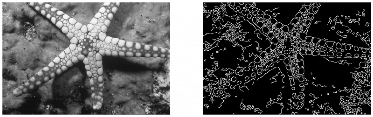
Figure 1.1 Edge Detection
Why Do We Need Edge Detection?
Discontinuities in depth, surface orientation, scene lighting changes, and variations in material properties can lead to discontinuities in image brightness. We obtain a set of curves representing object boundaries and surface markings, as well as curves corresponding to surface orientation discontinuities.
Therefore, applying edge detection algorithms to images can significantly reduce the amount of data to be processed, filtering out information that may be considered less relevant while retaining important structural properties of the image.
As shown in Figure 1.1, the structural properties of the image are captured through edge detection.
Understanding Popular Edge Detection Algorithms
After discussing the importance of edge detection algorithms, this section will focus on understanding some popular and widely used edge detection algorithms.
There are various methods for edge detection. Let’s roughly categorize these methods into:
- Traditional Methods
- Deep Learning-Based Methods
Now, let’s discuss one of the most popular edge detection algorithms—the Canny edge detector—and compare it with Sobel and Prewitt.
Canny Edge Detector
The Canny edge detection algorithm is widely used in today’s image processing applications. It works in multiple stages, as shown in Figure 1.2. The Canny edge detection algorithm produces smoother, thinner, and clearer images compared to Sobel and Prewitt filters.
Here is a summary of the Canny edge detection algorithm:
Smooth the input image and apply the Sobel filter to detect edges in the image. We then apply non-maximum suppression to retain local maximum pixels in the gradient direction, while suppressing the rest. We apply thresholding to remove pixels below a certain threshold and retain pixels above a certain threshold to eliminate edges that may have formed due to noise.
Later, if any of the 8 neighboring pixels is strong, we apply hysteresis tracking to strengthen the pixel.
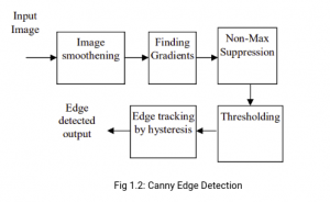
Figure 1.2 Canny Edge Detector
Now, we will discuss each step in detail.
Canny edge detection involves 5 steps, as shown in the above Figure 1.2. We will use the following images for illustration.
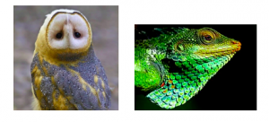
Image Smoothing
In this step, we convert the image to grayscale, as edge detection does not depend on color. We then use a Gaussian filter to remove noise from the image, as edge detection is sensitive to noise.
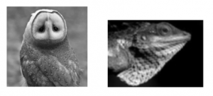
Finding the Intensity Gradient of the Image
Next, we apply the Sobel kernel in both horizontal and vertical directions to obtain the first derivatives in the horizontal direction (Gx) and vertical direction (Gy) of the smoothed image. We then calculate the edge gradient (G) and angle (θ) as follows:
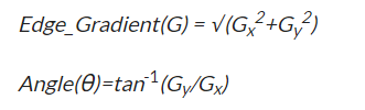
We know that the gradient direction is perpendicular to the edge. We round the angle to one of four angles representing vertical, horizontal, and two diagonal directions.
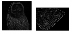
Non-Maximum Suppression
Now we remove all pixels that may not constitute edges. To do this, we check if each pixel is a local maximum in its neighborhood in the gradient direction. If it is a local maximum, it is considered for the next stage; otherwise, it is darkened and set to 0. This will give a thin line in the output image.
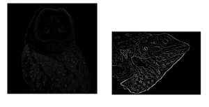
Double Threshold
Pixels caused by noise and color variation will persist in the image. Therefore, to eliminate this, we obtain two thresholds from the user, lowerVal and upperVal.
We filter out edge pixels with weak gradient values (lowerVal) and retain edge pixels with high gradient values (upperVal). Edges with intensity gradients greater than upperVal are certainly edges, while those below lowerVal are definitely non-edges, so they are discarded. Pixels with values less than upperVal and greater than lowerVal are considered part of the edge if they are connected to a “sure-edge.” Otherwise, they will also be discarded.
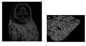
Hysteresis Edge Tracking
If any of the 8 neighboring pixels around a pixel is a strong pixel (pixel value = 255), it is set to a strong pixel; otherwise, it is set to 0.
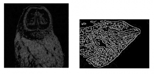
This is almost everything about Canny edge detection. As shown, edges are detected from the image.
Now, we will explore deep learning-based edge detection methods. But why do we need to use deep learning-based edge detection algorithms in the first place? Canny edge detection focuses only on local changes and does not understand the semantics of the image, that is, the content of the image. Therefore, deep learning-based algorithms were proposed to address these issues. We will now discuss it in detail.
But before we delve into the mathematics of deep learning, let’s first try to implement the Canny edge detector and the deep learning-based model (HED) in OpenCV.
Implementation – Canny Edge Detector
Let’s import the necessary modules
import cv2
from skimage.metrics import mean_squared_error, peak_signal_noise_ratio, structural_similarity
import matplotlib.pyplot as plt
The following code applies the Canny edge detector on the starfish image
img_path = 'starfish.png'
# Reading the image
image = cv2.imread(img_path)
(H, W) = image.shape[:2]
# convert the image to grayscale
gray = cv2.cvtColor(image, cv2.COLOR_BGR2GRAY)
# blur the image
blurred = cv2.GaussianBlur(gray, (5, 5), 0)
# Perform the canny operator
canny = cv2.Canny(blurred, 30, 150)
Let’s see the output of the Canny edge detector
fig, ax = plt.subplots(1, 2, figsize=(18, 18))
ax[0].imshow(gray, cmap='gray')
ax[1].imshow(canny, cmap='gray')
ax[0].axis('off')
ax[1].axis('off')
Next, let’s take a look at the HED code before doing the math.
Implementation – HED
# This class helps in cropping the specified coordinates in the function
class CropLayer(object):
    def __init__(self, params, blobs):
        # initialize our starting and ending (x, y)-coordinates of
        self.startX = 0
        self.startY = 0
        self.endX = 0
        self.endY = 0
    def getMemoryShapes(self, inputs):
        (inputShape, targetShape) = (inputs[0], inputs[1])
        (batchSize, numChannels) = (inputShape[0], inputShape[1])
        (H, W) = (targetShape[2], targetShape[3])
        # compute the starting and ending crop coordinates
        self.startX = int((inputShape[3] - targetShape[3]) / 2)
        self.startY = int((inputShape[2] - targetShape[2]) / 2)
        self.endX = self.startX + W
        self.endY = self.startY + H
        # return the shape of the volume (we'll perform the actual
        # crop during the forward pass
        return [[batchSize, numChannels, H, W]]
    def forward(self, inputs):
        return [inputs[0][:, :, self.startY:self.endY, self.startX:self.endX]]
You can download deploy.prototxt and caffemodel from this repo: https://github.com/ashukid/hed-edge-detector
# The caffemodel contains the model of the architecture and the deploy.prototxt contains the weights
protoPath = 'deploy.prototxt.txt'
modelPath = 'hed_pretrained_bsds.caffemodel'
net = cv2.dnn.readNetFromCaffe(protoPath, modelPath)
# register our new layer with the model
cv2.dnn_registerLayer("Crop", CropLayer)
Now we read our image and pass it to the algorithm.
# Input image is converted to a blob
blob = cv2.dnn.blobFromImage(image, scalefactor=1.0, size=(W, H), mean=(104.00698793, 116.66876762, 122.67891434), swapRB=False, crop=False)
# We pass the blob into the network and make a forward pass
net.setInput(blob)
hed = net.forward()
hed = cv2.resize(hed[0, 0], (W, H))
hed = (255 * hed).astype("uint8")
We read the actual image composed of edges
test_y_path = 'edge.png'
test_y = cv2.imread(test_y_path)
# The test image has its third dimension as 3
# So we are extracting only one dimension
test_y = test_y[:, :, 0]
We normalize the images so that MSE values do not rise
# Normalizing all the images
test_y = test_y / 255
hed = hed / 255
canny = canny / 255
gray = gray / 255
We now visualize our results
fig, ax = plt.subplots(1, 2, figsize=(18, 18))
ax[0].imshow(gray, cmap='gray')
ax[1].imshow(hed, cmap='gray')
ax[0].axis('off')
ax[1].axis('off')
Finally, we calculate metrics and compare our results
# Calculating metrics between actual test image and the output we got through Canny edge detection
print(mean_squared_error(test_y, canny), peak_signal_noise_ratio(test_y, canny), structural_similarity(test_y, canny))
# Calculating metrics between actual test image and the output we got through HED
print(mean_squared_error(test_y, hed), peak_signal_noise_ratio(test_y, hed), structural_similarity(test_y, hed))

Why Use Deep Learning for Edge Detection?
Before reading HED, a question may arise: why do we need deep learning algorithms to accomplish such a simple edge detection task?
The answer is that Canny edge detection primarily focuses on local changes rather than the semantics of the image, meaning it pays less attention to the content of the image. Therefore, we obtain less accurate edges.
Deep Learning Approaches to Edge Detection
The Holistically-Nested Edge Detection (HED) technique is a learning-based end-to-end edge detection system that uses a pruned VGG-like convolutional neural network to perform image-to-image prediction tasks. HED generates edge outputs within the neural network. All side outputs are fused together to form the final output. Let’s take a closer look at the algorithm.
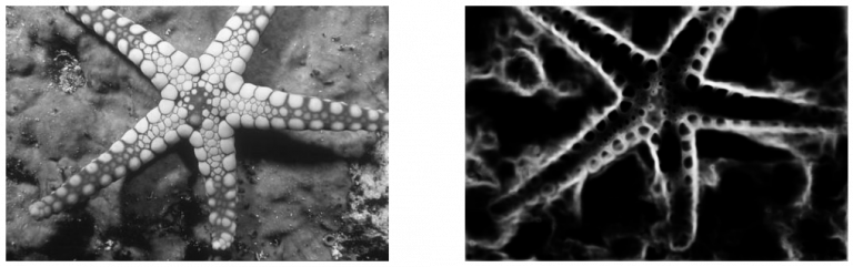
Figure 1.3 Edge Detection Using HED
Algorithm Overview
We adopt the VGGNet architecture but make the following modifications:
(a) We connect the side output layers to the last convolutional layer of each stage, which are conv1 2, conv2 2, conv3 3, conv4 3, and conv5 3.
(b) We remove the last stage of VGGNet, including the 5th pooling layer and all fully connected layers. Furthermore, the deconvolution layers within the network combine the output of bilinear interpolation.
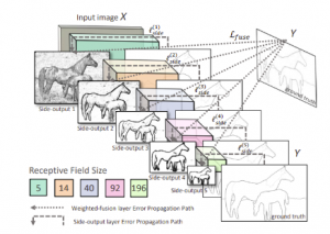
Figure 1.4: HED
The training and testing phases of HED will be covered in the last section of this article. I recommend you browse through it for a better understanding of the model architecture.
HED: Training and Testing Phases
Now, let’s talk about the training and testing phases of HED. As I mentioned at the beginning of the article, this is a section that involves a lot of mathematical knowledge, so reading this part is optional. I strongly encourage you to read this section to truly grasp the inner workings of HED.
Training Phase
Let us denote the set of all standard network layer parameters as W, which has M side output layers. Each side output layer is also associated with a classifier, with the corresponding weights denoted as w = (w (1), . . . , w (m)).

Where lside represents the image-level loss function of the side output. For typical natural images, there is a severe imbalance in the distribution of edge/non-edge pixels: 90% are non-edges. A cost-sensitive loss function introduces an additional weighting parameter for biased sampling.
Specifically, we define the following class-balanced cross-entropy loss function used in the above equation.
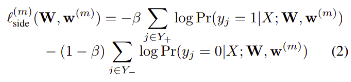
Where:
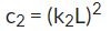
k1 = 0.01 and k2 = 0.03

Testing Phase
During testing, given an image X, we obtain edge map predictions from the side output layer and the weighted fusion layer. The final unified output can be obtained by aggregating these generated edge maps.
Evaluation Metrics
Now that we have covered different edge detection algorithms—traditional and deep learning methods. But how do we evaluate the performance of edge detection algorithms or compare different edge detection algorithms?
This brings us to another interesting topic in edge detection—evaluation metrics. We will now discuss various evaluation metrics for edge detection.
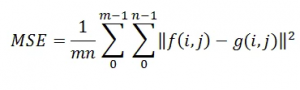
Mean Squared Error
MSE measures the ability of distortion noise to affect the quality of representation.
Formula:
Peak Signal to Noise Ratio Equation
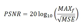
Peak Signal to Noise Ratio (PSNR) indicates the ratio between the maximum possible value (power) of a signal and the power of distortion noise affecting its representation quality. It is given by
Structural Similarity Index Measure
Structural Similarity Index Measure extracts three key features from the brightness, contrast, and structure of the image. Formula:

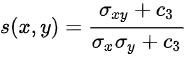
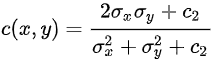
Where:
μx is the average of image X
μy is the average of image Y
 is the variance of X
 is the variance of Y
 is the covariance of X and Y
 and
and
k1 = 0.01 and k2 = 0.03
Conclusion
We have covered all concepts of the Canny edge detector and coded it using OpenCV. We discussed the 5 steps involved in Canny edge detection and why the Canny edge detector is better than previous methods. We also introduced the mathematics involved in the HED method. We discussed some evaluation metrics to assess the algorithm’s performance on images.
The main points of this article are:
- The Canny edge detector provides smoother and finer edges than Sobel and Prewitt filters
- A deep learning method that focuses on the content of the image
Download 1: OpenCV-Contrib Extension Module Chinese Tutorial

Reply "OpenCV Extension Module Chinese Tutorial" in the "Beginner Learning Vision" public account to download the first Chinese version of the OpenCV extension module tutorial available on the internet, covering more than twenty chapters including extension module installation, SFM algorithms, stereo vision, object tracking, biological vision, super-resolution processing, etc.

Download 2: 52 Lectures on Python Vision Practical Projects

Reply "Python Vision Practical Projects" in the "Beginner Learning Vision" public account to download 31 visual practical projects, including image segmentation, mask detection, lane line detection, vehicle counting, eyeliner addition, license plate recognition, character recognition, emotion detection, text content extraction, face recognition, etc., to help quickly learn computer vision.

Download 3: 20 Lectures on OpenCV Practical Projects

Reply "OpenCV Practical Projects 20 Lectures" in the "Beginner Learning Vision" public account to download 20 practical projects based on OpenCV, achieving advanced learning in OpenCV.

Group Chat

Welcome to join the reader group of the public account to communicate with peers. Currently, there are WeChat groups for SLAM, 3D vision, sensors, autonomous driving, computational photography, detection, segmentation, recognition, medical imaging, GAN, algorithm competitions, etc. (will gradually be subdivided in the future). Please scan the WeChat number below to join the group, and note: "Nickname + School/Company + Research Direction", for example: "Zhang San + Shanghai Jiao Tong University + Vision SLAM". Please follow the format for notes; otherwise, you will not be approved. Once added successfully, you will be invited into the relevant WeChat group based on your research direction. Please do not send advertisements in the group; otherwise, you will be removed from the group. Thank you for your understanding~