IntroductionThe author has previously been learning communication algorithms through MATLAB simulations and has recently started to learn how to implement the communication systems constructed in MATLAB simulations using FPGA. Due to the significant differences between MATLAB simulation code and Verilog code, and the unfamiliarity with FPGA implementations of communication systems, the author decided to write an article documenting the experimental process. This serves as a personal note and, if it helps readers in their learning and thinking, it will be considered a success. As a start, let us begin with the most basic BPSK modulation method and first familiarize ourselves with how the fundamental modules in the communication process are implemented.PART0 Overall Design and Parameter DescriptionAs the most basic BPSK modulator and demodulator, the signal transmission from generation to reception and decision-making consists mainly of the following fundamental processes: First, construct a binary transmission signal and perform bipolar transformation; then upsample the signal to match the subsequent sampling frequency; the signal undergoes roll-off filtering through a root raised cosine filter; the signal is multiplied by a carrier for upconversion; it is then multiplied by the carrier again for downconversion; and finally, it passes through the root raised cosine filter again; downsample for symbol decision. For this initial experiment, we will temporarily ignore modules such as channel noise, carrier synchronization, bit synchronization, channel equalization, and encoding/decoding.In the specific FPGA implementation of the basic BPSK modulator and demodulator, the related modules of the transmitter and receiver form a symmetrical structure, with upconversion, filtering, and upsampling/downsampling having similar structures. If we can complete the implementation of the transmitter, then the receiver will be straightforward. Therefore, this article mainly focuses on the explanation of the transmitter, and the related modules of the receiver can refer to the structure of the transmitter for implementation.The specific experimental design and parameter description for this experiment are as follows:All signal transmissions in the experiment are accompanied by a valid line, where a high level indicates that the data on the signal line is valid. All signal lines are signed types. The top-level transmitter module (bpsk.v) connects sequentially to the bipolar transformation and upsampling (bipolar_signal.v), roll-off filtering (rcos_filter.v), and upconversion (up_conversion.v) modules. In the testbench, the bipolar transformation and upsampling module will receive data at a symbol rate of 10000 bit/s for a total duration of 1 second. The overall system clock used is clk=100MHz.The bipolar transformation and upsampling module will perform oversampling with sps=16, and the filter coefficients required for the rcos_filter.v module are generated by MATLAB. The cosine carrier required for the upconversion module is generated using the DDS IP core in Vivado. Other specific parameters and overall simulation design can be referenced in the appendix at the end.PART1 Testbench File DesignThe testbench file will open the msg_data.txt file, read the data, and send 1 second of data to the bipolar transformation and upsampling module at a rate of 10000 bit/s.
// Open the file and read datafile = $fopen("msg_data.txt", "r");if (file == 0) begin $display("Failed to open the file!"); $finish;end // Read data from the file and pass it to the modulei = 0;flag = 1;while (!$feof(file) && (flag == 1)) begin $fscanf(file, "%d\n", msg_input); // Read each line of data from the file msg_data = msg_input; // Pass the data to msg_data // Set top_valid to 1 each time data is passed, indicating data is valid top_valid = 1; #100000; // Wait for one clock cycle i = i + 1; if (i == 10000) begin flag = 0; endendtop_valid = 0;PART2 Bipolar Transformation and Upsampling Module(bipolar_signal.v) The module interface is as follows:
input clk, // Clock signal, period 10nsinput reset, // Reset signalinput [7:0] msg_data, // 8-bit input messageinput top_valid, // Valid signal from the top layeroutput reg signed [1:0] bipolar_signal, // Bipolar signal output, using 2-bit signed typeoutput reg valid // Valid signalThe experiment requires two counters: one is the sample point period counter sample_counter, which has a period of 6250ns for a single sample point, i.e., 625 clock cycles; the other is the counter for each symbol’s sample points signal_counter, with a maximum value of 16 for each symbol’s samples, incrementing by 1 each time sample_counter counts to 625-1.The operation of this module mainly relies on these two counters. For the output signal line bipolar_signal, we only need to perform bipolar transformation on the msg_data line data each time signal_counter is 0; at other times, it can remain 0. For the output valid line, it is pulled high when the first data is sent and pulled low 6250ns after the last data is sent. This logic will be used for subsequent modules, and will not be repeated for other valid lines.
// Determine output based on signal_counter valueif (signal_counter == 0) begin // Output original bipolar signal for the first sample point if (top_valid == 0) begin end if (msg_data == 8'b00000001) begin if(top_valid != 0 ) bipolar_signal <= 1; // +1 end else begin if(top_valid != 0 ) bipolar_signal <= -1; // -1 endend else begin // Output zero interpolation for the next 15 sample points bipolar_signal <= 0;endPART3 Roll-off Filter Module(rcos_filter.v) The module interface and some variables are as follows:
input clk, // Clock signalinput reset, // Reset signalinput signed [1:0] bipolar_signal, // Input bipolar signalinput valid, // Input signal valid flagoutput reg signed [19:0] filtered_signal, // Output filtered signal, 20-bit signed typeoutput reg valid_out // Filter output valid signal// Storage for filter coefficients, length 97, 20-bitreg signed [19:0] rcos_fir[0:96]; // Filter coefficients, 20-bitreg signed [19:0] shift_reg[0:96]; // Filter state register, 20-bitreg [9:0] receiver_counter; // Counter for synchronizing received dataFirst, we need to complete the task of generating filter coefficients from MATLAB. This will facilitate the import of coefficients into the module.In MATLAB, the coefficients of the root raised cosine filter can be generated using the rcos_fir function, but the generated coefficients are less than 1, which is clearly unsuitable for Verilog implementation. Therefore, after generation, we first need to perform a scaling operation to convert them into integers.Secondly, in Verilog, reading a txt file is mainly done using the readmemh and readmemb functions. Here, we will use the readmemb function, so we need to convert the decimal coefficients into binary coefficients.Additionally, since we use signed variables in Verilog, we also need to perform two’s complement processing for negative numbers.The code can be found in the appendix at the end.To synchronize the received bipolar_signal from the bipolar transformation and upsampling module, we need a receiver_counter. We set this module to have a 3us delay for data reception and transmission. Each time the counter counts to 300, this time is in the middle of the duration of each data on the data line, as shown in the figure below. It can be seen that the change moment of filtered_signal is in the middle of the two change moments of the bipolar_signal signal. At this time, the roll-off filter module receives the bipolar signal data and performs convolution processing. How to implement convolution processing in Verilog? First, we design an input signal register array with a length of [0:96]. Each time a bipolar signal is received, the register shifts up by one position, and then the current bipolar signal is inserted into the lowest position of the register. The output signal is composed of the current signal multiplied by the first coefficient of the filter, plus the previous signal multiplied by the second coefficient of the filter, plus the signal before that multiplied by the third coefficient of the filter, and so on, to synthesize the output signal.
// Synchronize data reception every 625 clock cycles (6250ns)if (receiver_counter == 300) begin // Update state register at the reception point for (i = 96; i > 0; i = i - 1) begin shift_reg[i] <= shift_reg[i - 1]; // Shift state register right end shift_reg[0] <= bipolar_signal; // Insert current signal if(!valid) begin // If valid is low, keep output zero filtered_signal <= 0; valid_out <= 0; // Output invalid signal end endif (receiver_counter == 301) begin // Convolution calculation: convolve values in shift_reg with rcos_fir coefficients filtered_signal = 0; // Clear current filtered signal for (i = 0; i < 97; i = i + 1) begin filtered_signal = filtered_signal + (shift_reg[i] * rcos_fir[i]); end // Set valid_out signal high to indicate output is valid valid_out <= 1; endPART4 Upconversion Module(up_conversion.v) The main function of this part is to multiply the filtered signal with the carrier. First, we design an IP core to generate the carrier signal.The dds_compiler IP core outputs a cosine wave with a fixed frequency and initial phase in this experiment, but the parameters set by the author are variable at any time. This allows us to introduce how to control frequency and phase. The two parameters related to the frequency control word and phase control word are shown in the figure below: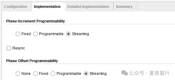 By referring to the IP core user manual, we can see that these two control words are controlled by the s_axis_phase_tdata data line. When both PINC and POFF are set to Streaming, the high bits of the data line control POFF, and the low bits control PINC.
 The calculations for the frequency control word and phase control word are:
 Where N is the Phase Width, which is the item in the Hardware Parameters section of the IP core parameter settings page.
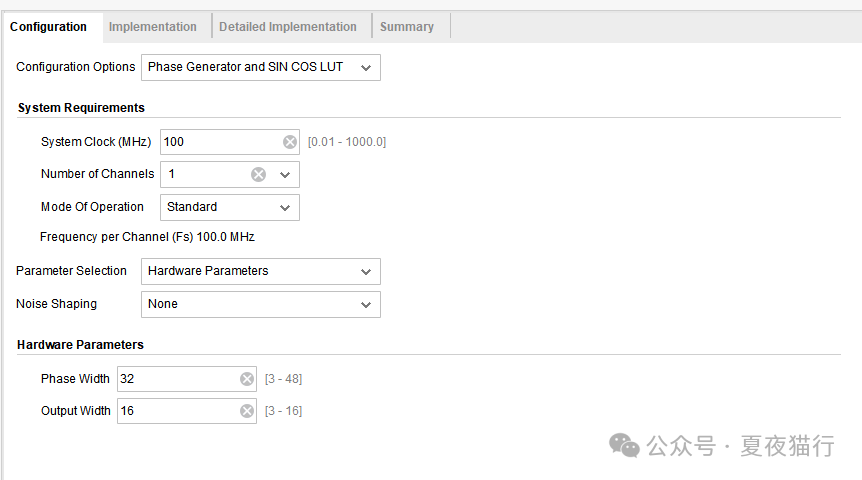 In the code, we only need to set it as shown in the figure below to control frequency and phase. In this experiment, we generate a cosine wave of 10000Hz with an initial phase of 0.
S_AXIS_PHASE_0_tdata[31:0] = 32'd429496; S_AXIS_PHASE_0_tdata[63:32] = 32'd0;After setting the IP core, we generate the top-level file and instantiate it in the upconversion module. We still use a similar code structure as in the roll-off filter module to implement data processing: using a counter to synchronize the reception of the filtered signal, setting a 3us delay, and performing the multiplication operation of the filtered signal with the carrier each time the counter counts to 300.However, if you directly use the cosine wave signal output from the IP core for multiplication, you will definitely find that there is a problem. The multiplication result does not meet expectations. What is the reason? The author discovered through debugging that the data output from the IP core is in two’s complement format, but the data line output from the IP core is unsigned. Because of this reason, when multiplying the signed filtered_signals with it directly, the code will incorrectly interpret the carrier’s two’s complement data as unsigned.To solve this problem, we can set another signed reg variable to store the original carrier signal in two’s complement format.
reg signed [34:0] filtered_signal_35;reg signed [34:0] M_AXIS_DATA_0_tdata_35;always@(*) filtered_signal_35 = filtered_signal;always@(*) M_AXIS_DATA_0_tdata_35 = {{19{M_AXIS_DATA_0_tdata[15]}},M_AXIS_DATA_0_tdata};The structure of the code for synthesizing the output signal is similar to that of the roll-off filter module:
// Update counterif (counter == 625 - 1) begin counter <= 0;end else begin if (valid_out || flag == 1) counter <= counter + 1;endif(!valid_out && counter == 300) begin flag <= 0; valid_up_signal <= 0;endif (counter == 300 && valid_out) begin // Signal multiplication: multiply filtered_signal and cosine wave signal generated by DDS up_signal <= filtered_signal_35 * M_AXIS_DATA_0_tdata_35; // Multiply cosine wave with filtered_signal valid_up_signal <= 1;endPART5 Simulation and ConclusionThrough the implementation of the above modules, we conducted simulations and observed very good results.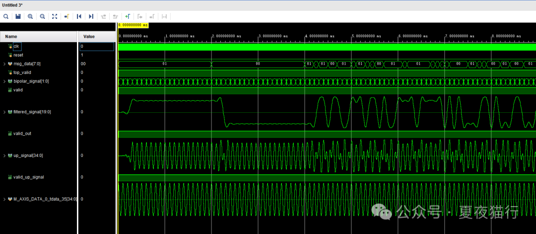 This experiment mainly focuses on how to conduct joint experiments with Vivado and MATLAB. It discusses how to process the data generated in MATLAB to make it suitable for FPGA implementation, how to export data, how to import data in Verilog, and how to use the DDS IP core. It also covers how to design a BPSK communication modulator and demodulator suitable for FPGA implementation, how to implement the structure of each communication module from MATLAB to FPGA, and how to write it in Verilog. These are all worth summarizing.The above is the complete content of this experiment. The MATLAB files can be referenced in the appendix below for further learning. I hope this can help readers, and goodbye~Appendix: MATLAB Simulation Files for BPSK ModulatorThis appendix will provide the MATLAB simulation code corresponding to the experiment, as well as the code for generating and exporting the transmitted signal and filter coefficients.
%%%%%%%%%%%%%%%%%%%%%%%%%%%% BPSK Transceiver System Simulation %%%%%%%%%%%%%%%%%%%%%%%%%%%%
clc;clear;tic;
%******** Parameter Settings ********%
% The FPGA clock is set to 100M, i.e., 10ns
% The binary data on the MATLAB side is sent at 10000 data per second in the testbench
% Each symbol will be sampled 16 times, i.e., each sample point is 6250ns
% The expected carrier has a period of 100us
bit_rate = 10000; % Bit rate
symbol_rate = 10000; % Symbol rate
sps = 16; % Number of sample points per symbol
fc = 10000; % Carrier frequency
fs = 160000; % Sampling frequency
rollof_factor = 0.5; % Roll-off factor
%******** PART0: Construct Binary Transmission Sequence (This part is generated using MATLAB and then imported into Vivado) ********%
% Construct signal sequence
msg_source = [ones(1,20) zeros(1,20) randi([0 1],1,9960)];
%******** PART1: Data Processing of the Transmitter ********%
% Perform bipolar transformation on the signal
bipolar_msg_source = 2*msg_source-1; % Bipolar signal
%******** PART2: Bipolar Signal Through Shaping Filter ********%
% First, upsample to match the subsequent sampling frequency
up16_bipolar_msg_source = upsample(bipolar_msg_source,sps);
% Construct root raised cosine shaping filter
rcos_fir = rcosdesign(rollof_factor,6,sps);
% Roll-off filtering
rcos_msg_source = filter(rcos_fir,1,up16_bipolar_msg_source);
% % Waveform observation
% figure(1);
% plot(rcos_msg_source);
% title('Time Domain Waveform');
% figure(2);
% plot(abs(fftshift(fft(rcos_msg_source))));
% title('Frequency Domain Waveform');
%******** PART3: Upconversion (Multiply by Carrier) ********%
time = [0:length(rcos_msg_source)-1]+0.45;
rcos_msg_source_carrier = rcos_msg_source.*cos(2*pi*fc.*time/fs);
% % Waveform observation
% figure(3);
% plot(rcos_msg_source_carrier);
% title('Time Domain Waveform');
% figure(4);
% plot(abs(fft(rcos_msg_source_carrier)));
% title('Frequency Domain Waveform');
%******** PART4: Downconversion: Multiply by Carrier ********%
rcos_msg_source_receive = rcos_msg_source_carrier.*cos(2*pi*fc.*time/fs);
% % Waveform observation
% figure(7);
% plot(rcos_msg_source_addnoise);
% title('Time Domain Waveform');
% figure(8);
% plot(abs(fft(rcos_msg_source_addnoise)));% title('Frequency Domain Waveform');
% Downconversion filtering
fir_lp = fir1(128,0.2);
rcos_msg_source_lp = filter(fir_lp,1,rcos_msg_source_receive);
% % Waveform observation
% figure(9);
% plot(rcos_msg_source_lp);
% title('Time Domain Waveform');
% figure(10);
% plot(abs(fft(rcos_msg_source_lp)));% title('Frequency Domain Waveform');
%******** PART5: Signal Through Matched Filter ********%
rcos_fir = rcosdesign(rollof_factor,6,sps);
% Filtering
rcos_msg_source_MF = filter(rcos_fir,1,rcos_msg_source_lp);
% % Waveform observation
% figure(11);
% plot(rcos_msg_source_MF);
% title('Time Domain Waveform');
% figure(12);
% plot(abs(fft(rcos_msg_source_MF)));% title('Frequency Domain Waveform');
%******** PART6: Sampling/Decision ********%
% Find the best sampling point
decision_site = 160; % Three filter delays 96 128 96, (96+128+96)/2=160
% Extract, select one point for decision every 1 symbol (every 16 sample points)
rcos_msg_source_MF_option = rcos_msg_source_MF(decision_site:sps:end);
% Decision
cos_msg_source_MF_option = sign(rcos_msg_source_MF_option);
% % Waveform observation
% figure(13);
% plot(cos_msg_source_MF_option,'-*');
% figure(14);
% plot(bipolar_msg_source,'-*');
% title('Time Domain Waveform');
[error_number,bit_err_ratio]=biterr(msg_source(1:length(rcos_msg_source_MF_option)),(1+cos_msg_source_MF_option)/2);
toc;
%%%%%%%%%%%%%%% Output signal to txt file
% Save as txt file, data stored as one bit per line
fileID = fopen('msg_data.txt', 'w');  % Open file
for i = 1:10000    fprintf(fileID, '%d\n', msg_source(i));  % Write each bit
endfclose(fileID);  % Close file
disp('Data has been saved as msg_data.txt');
%%%%%%%%%%%%% Output rcos to txt file
% MATLAB code: Generate coefficients of the root raised cosine filter and save them as integers in txt file
% Filter parameters
rolloff_factor = 0.5;  % Roll-off factor
span = 6;              % Filter length (in symbols)
sps = 16;              % Number of sample points per symbol
% Generate root raised cosine filter
rcos_fir = rcosdesign(rolloff_factor, span, sps);
% Scale coefficients
scaling_factor = 1000000;
rcos_fir_scaled = round(rcos_fir * scaling_factor);
% Assume using 20-bit binary representation for filter coefficients (adjust bit width as needed)
bitwidth = 20;
% Open file and save in signed binary format
fileID = fopen('rcos_fir_scaled.txt', 'w');  % Open file
for i = 1:length(rcos_fir_scaled)    % Get binary representation of each signed integer    if rcos_fir_scaled(i) < 0        % Perform two's complement processing for negative numbers        bin_str = dec2bin(2^bitwidth + rcos_fir_scaled(i), bitwidth);  % Two's complement representation    else        % Positive numbers directly converted to binary        bin_str = dec2bin(rcos_fir_scaled(i), bitwidth);    end    % Write binary string to file    fprintf(fileID, '%s\n', bin_str);endfclose(fileID);  % Close file
disp('Filter coefficients have been saved in signed binary format to rcos_fir_scaled.txt');