In a previous article, we discussed linear interpolation. Today, we will talk about arc interpolation. While linear interpolation is based on three-dimensional space (three axes), here we will focus on arc interpolation in two-dimensional space (two axes).
1. Schematic Diagram
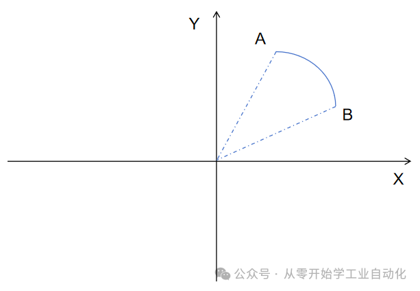
In a plane, our robotic arm needs to move from point A to point B (for process requirements, such as applying glue along the circular edge of a product). At this point, we will utilize the arc interpolation function.
2. Implementation Principle
First, we need to understand that the arc trajectory is achieved through two motion axes, typically the X-axis and Y-axis, or a rotational axis. Here, we will mainly explain how to implement the principle of arc interpolation using the X-axis and Y-axis. It primarily generates a series of continuous and smooth “micro line segments” to ultimately create an arc path that meets precision requirements.
The PLC itself is not designed for motion control. The true principle of implementing arc interpolation is through software algorithms that calculate the coordinates of trajectory points, converting these coordinate values into control signals for the drive system (such as stepper or servo motors) to achieve synchronized displacement of the two axes, thus tracing the arc trajectory.
3. Mathematical Foundation
Any arc can be defined by its center coordinates (X₀,Y₀), radius, starting angle θ₁, and ending angle θ₂. Alternatively, it can be defined by the center coordinates (X₀,Y₀), starting point (X₁,Y₁), and ending point (X₂,Y₂). Its mathematical equation is:
(X – X₀)² + (Y – Y₀)² = R²However, our PLC cannot directly recognize continuous equations; it must discretize the arc into countless “micro line segments” as interpolation points. For every small angle Δθ or small displacement ΔL, a specific (Xᵢ,Yᵢ) coordinate point is calculated, and then the two axes are controlled to move from the current point to the next interpolation point.The discretization accuracy is determined by two parameters: the “interpolation period T” and the “small increment Δ”: the interpolation period T is the time interval for the PLC to calculate the next interpolation point (usually 1ms to 10ms, which needs to match the response speed of the drive system); the small increment Δ is the minimum distance the two axes move within each cycle, for example, 0.01mm. The smaller Δ is, the smoother the arc fitting and the higher the accuracy.Does it seem a bit confusing? It’s the same for everyone.4. The Most Common Arc Interpolation Algorithm Used in PLC: Point-by-Point Comparison MethodLastly, after discussing this, you can try it out; we won’t implement the program here.Due to the generally limited computation speed and memory of PLCs, simpler, real-time algorithms that do not require complex floating-point calculations are often chosen. Among them, the “point-by-point comparison method” is the most common arc interpolation algorithm in the industry. The principle can be summarized as: at each step, check the deviation and correct the direction. This is specifically divided into four steps that are executed in a loop:1. Calculate Deviation: Determine the relationship between the current position and the arc
We first define the “deviation function F” to determine whether the current position of the two axes controlled by the PLC (Xᵢ,Yᵢ) is on the arc, inside the arc, or outside the arc:
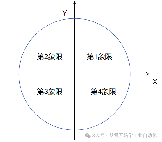
Taking the “first quadrant counter-arc” (the clockwise/counterclockwise direction only affects the direction, the logic remains consistent) as an example, with the center at the origin (X₀=0,Y₀=0) and radius R, the deviation function is:
Fᵢ = Xᵢ² + Yᵢ² – R²
- If Fᵢ = 0: The current point is on the arc, so the next step can move along the X or Y axis (depending on the interpolation direction);
- If Fᵢ > 0: The current point is outside the arc, so the next step needs to move inward (usually decrease the X-axis, i.e., Xᵢ₊₁ = Xᵢ – Δ);
- If Fᵢ < 0: The current point is inside the arc, so the next step needs to move outward (usually increase the Y-axis, i.e., Yᵢ₊₁ = Yᵢ + Δ).
A key optimization is:Calculating the square directly in the PLC is computationally intensive. To reduce the computational load, we can derive the relationship between Fᵢ₊₁ and Fᵢ using its “recursion formula” as follows:
- If moving in the negative direction on the X-axis (Xᵢ₊₁ = Xᵢ – Δ), then Fᵢ₊₁ = Fᵢ – 2ΔXᵢ + Δ²;
- If moving in the positive direction on the Y-axis (Yᵢ₊₁ = Yᵢ + Δ), then Fᵢ₊₁ = Fᵢ + 2ΔYᵢ + Δ²;
Through recursion, the PLC only needs to perform addition and subtraction, greatly enhancing our real-time performance.
2. Movement Control: Drive the two axes to the next interpolation point
Based on the deviation calculation results, the PLC sends “displacement commands” to the drive systems (servo/stepper drivers) of the X and Y axes:
- If we need to move the X-axis: we send the corresponding number of “pulses” through the PLC pulse output (e.g., Mitsubishi FX5U’s Y0/Y1) (pulse count = Δ/pulse equivalent, for example, if the pulse equivalent is 0.001mm, then Δ=0.01mm requires 10 pulses), while setting the movement direction (positive/negative) through the direction port (e.g., Y2/Y3);
- If we need to move the Y-axis: similarly, send signals to the pulse and direction ports of the Y-axis;
- Special case (Fᵢ=0): Based on the direction of arc interpolation (clockwise/counterclockwise), preset its priority, for example, counter-arc prioritizes moving along the X-axis, while clockwise prioritizes moving along the Y-axis, etc.
3. Determine Endpoint: Check if the arc has reached the endpoint
Our PLC needs to determine in real-time whether the current interpolation point is close to or has reached the arc endpoint (X₂,Y₂). Two commonly used methods for this determination are:
Total Steps Judgment: Pre-calculate the total number of interpolation steps N corresponding to our arc (N = arc length/Δ). Count down by one for each step taken, and when the count reaches 0, stop the interpolation;
- Coordinate Comparison Judgment: Real-time compare the current Xᵢ with the endpoint X₂ and Yᵢ with the endpoint Y₂. When |Xᵢ – X₂| ≤ Δ and |Yᵢ – Y₂| ≤ Δ, determine that the endpoint has been reached and stop pulse output. This method is relatively simple.
4. Loop Execution: Until the arc trajectory is completed
Our PLC can use “timer interrupts” or “scan cycle synchronization” to loop through the previous three steps: “deviation calculation → movement control → endpoint judgment”. Each PLC scan cycle generates one interpolation point, and the two axes (X and Y) move synchronously. Ultimately, countless micro line segments will create a continuous arc, and the task is complete.
5. Conclusion
First, it is essential to understand the mathematical foundation and implementation principles before considering how our PLC can achieve this. A critical point to note is: it must be done using interrupts; otherwise, the effect of implementation will be limited by the scan cycle. Everyone should try simulating this with a PLC.
If anyone has questions or needs to discuss, feel free to leave a comment. If you like it, please give a thumbs up and follow, or save it for later.Here are related series of learning articles:Beginner Project [Automatic Screw Machine] C#, PLC, Touch Screen Practical (1/5): Electrical Preliminary DesignEssential for Electrical Newbies! Quick Start PLC Projects: Detailed Breakdown of 7 Steps!
Beginner Project [OpenCV Visual Sorting Robot Arm] (1/3): Solution Design. [C# Winforms, OpenCV Vision, PLC Practical]