Using Oscilloscope with Cost-Effective EtherCAT Motion Controller

XPLC006E Function Overview

0

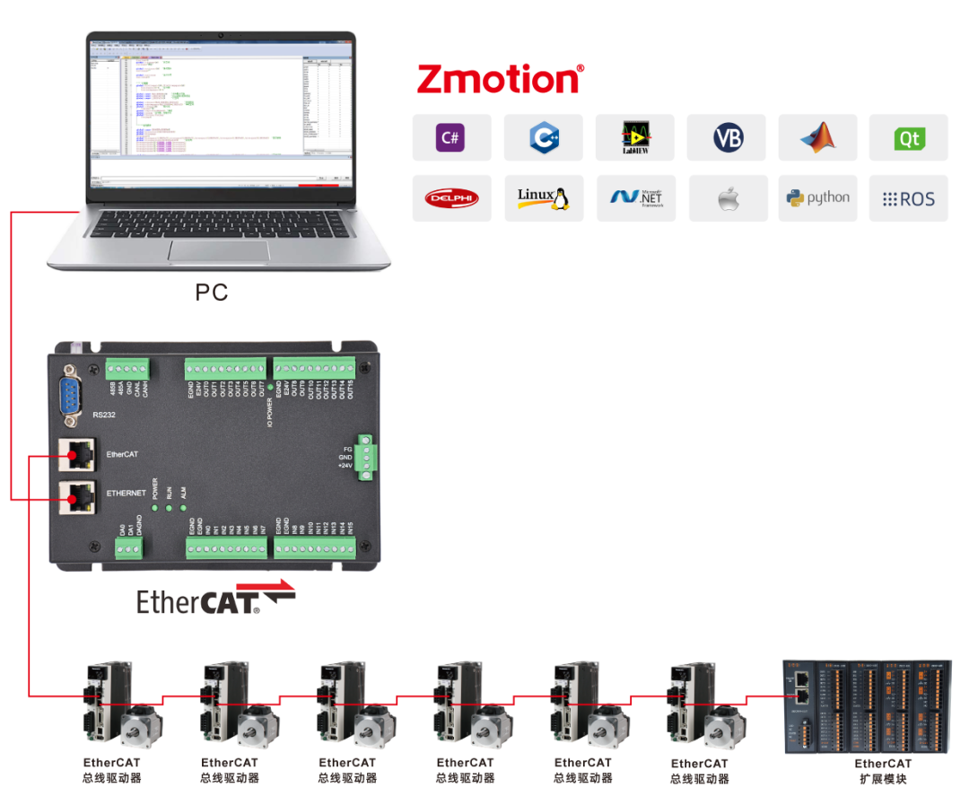
XPLC006E is a multi-axis cost-effective EtherCAT bus motion controller launched by Zheng Motion. The XPLC series motion controllers can be used in various scenarios that require offline or online operation.

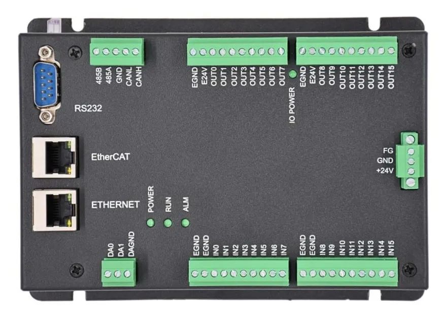
XPLC006E comes with 6 motor axes and supports up to 12 axes of motion control (including virtual axes), supporting 12-axis linear interpolation, electronic cam, electronic gear, synchronous tracking, virtual axis settings, and other functions.

XPLC006E supports multi-tasking operations simultaneously and can be directly simulated and run on a PC. It offers various programming options, supporting Basic/PLC ladder diagram/HMI configuration using ZDevelop software and common upper computer software programming.

XPLC006E only supports EtherCAT bus axes and does not support pulse axes and encoder axes. It communicates with drivers via EtherCAT bus with a refresh cycle of 1ms.

XPLC006E supports three programming methods: PLC, Basic, and HMI configuration. PC upper computer API programming supports interfaces like C#, C++, LabVIEW, VB, Matlab, Qt, Linux, .Net, iMAC, Python, ROS, etc.

→ This product has three different models available: XPLC004E, XPLC006E, and XPLC008E with varying numbers of axes.

2

2

XPLC864E Function Overview

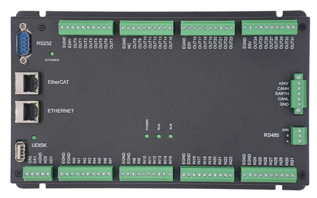
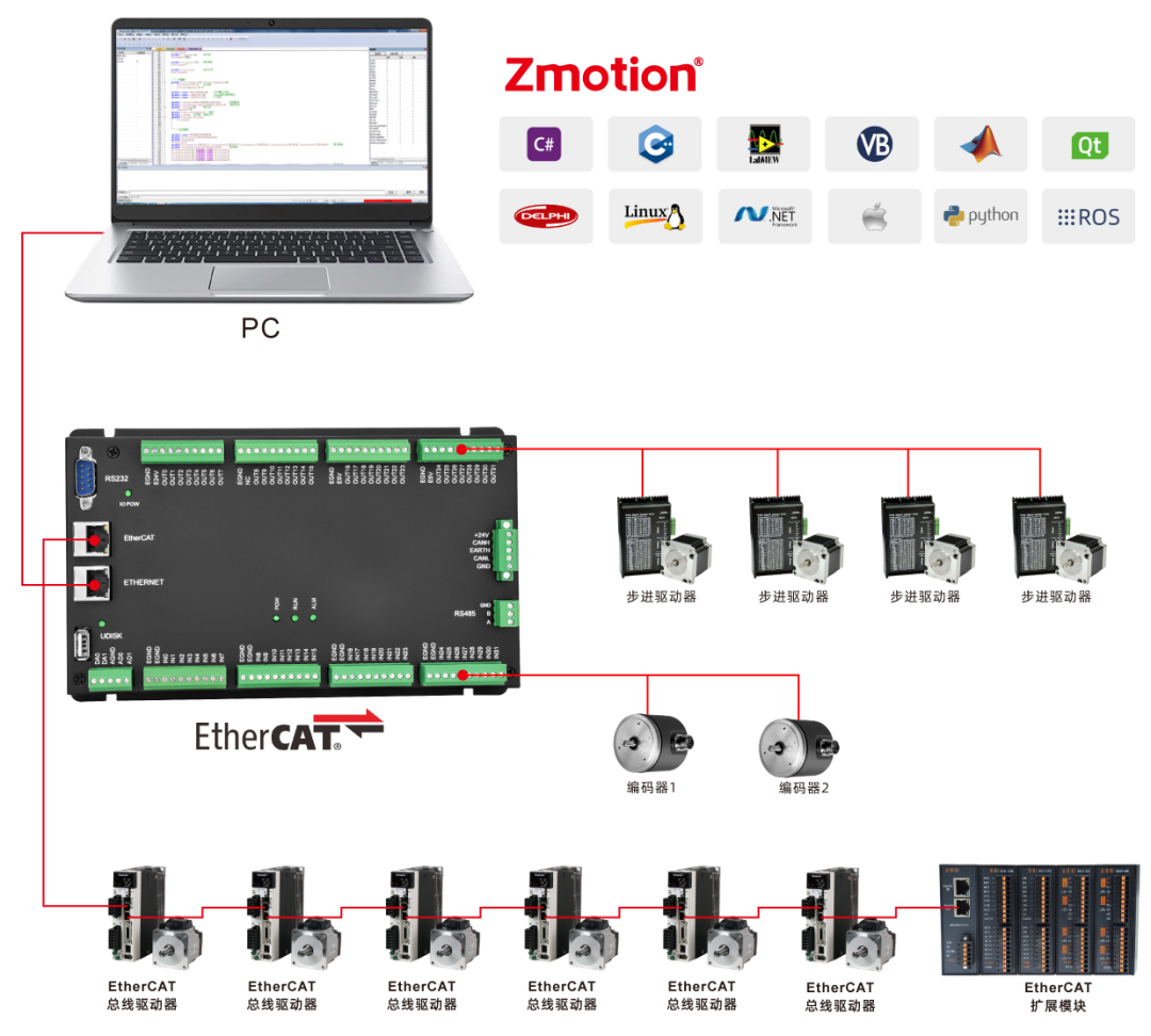
XPLC864E is an upgraded version of XPLC006E (the functions introduced in the previous section are all supported), with some resource space superior to XPLC006E. The usage method is basically the same, but the difference is that XPLC864E hardware supports 32 input points, 32 output points, 2 ADCs, and 2 DACs, supporting mixed use of pulse axes and bus axes, with a total of 8 actual axes. In addition to having an EtherCAT interface, the output ports can be configured to output pulse direction signals for 8 axes, and it also has two encoder inputs that can be configured from the input ports.

XPLC864E supports three programming methods: PLC, Basic, and HMI configuration. PC upper computer API programming supports C#, C++, LabVIEW, VB, Matlab, Qt, Linux, .Net, iMAC, Python, ROS, and other interfaces.

2

2

XPLC series cost-effective EtherCAT bus motion controllers support various programming methods and support the use of the ZDevelop development environment independently developed by Zheng Motion with Basic language and PLC ladder diagrams. The previous section explained the controller’s axis parameters and motion command descriptions, while this section mainly explains the use of the controller’s oscilloscope.

1

Function of the Oscilloscope

The oscilloscope is an extremely important part of program debugging and operation, used to convert signals that are invisible to the naked eye into graphics, facilitating the study of various signal changes, such as the current speed and position changes of the axis.

The oscilloscope uses data processed internally by the controller to obtain the current value of the data at regular intervals, and then displays all values obtained as a graph that changes over time. The oscilloscope can display various different signals, such as axis parameters, axis status, etc.

In the “View” → “Oscilloscope”, open the oscilloscope window, as shown in the figure below.

⊙ The oscilloscope must be started and then triggered to successfully sample. After opening the oscilloscope and setting the relevant parameters, click “Start”. You can click “Manual Trigger” to sample, or you can add the “TRIGGER” command in the program to automatically trigger the oscilloscope sampling.

2

Oscilloscope Panel Introduction

1. Main Interface

The button functions of the oscilloscope main interface are explained.

(1) Basic Settings

Settings: Open the oscilloscope settings window to set the relevant parameters of the oscilloscope.

Start: Start the oscilloscope (indicating that the oscilloscope is ready and waiting for trigger sampling).

Stop: Stop the oscilloscope sampling.

Horizontal Scale: The scale of one grid on the horizontal axis (time) in YT mode; this parameter is invalid in other modes.

<<: Press to hide channel names and peak displays, showing only channel numbers.

Continuous Sampling: When continuous sampling is not enabled, sampling will stop after reaching the sampling depth. When continuous sampling is enabled, the oscilloscope will continuously sample.

Follow: When following is enabled, the horizontal axis will automatically move to the real-time sampling position, displaying the follow waveform.

Manual Trigger: Manual trigger oscilloscope sampling button (automatic trigger uses the TRIGGER command).

Import/Export: Export the sampled data points from the oscilloscope to a txt file; to reload and display, click import; detailed instructions will be given in the next section.

(2) Display Mode

YT Mode: Curves of different data sources changing over time.

XY Mode: Displays the composite trajectory of two axes in a certain plane, combining the curves of the first and second channels, suitable for two-axis interpolation.

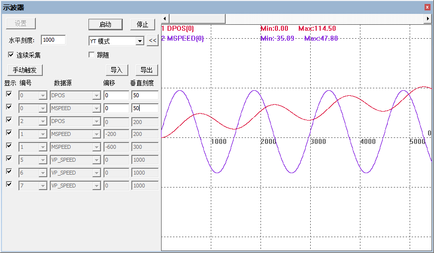
(3) Sampling Data Settings

Display: Choose whether to display the current channel curve.

Number: Select the data source number to be sampled, referring to data sources such as: axis number, digital IO number, analog IO number, TABLE number, VR number, MODBUS number, etc.

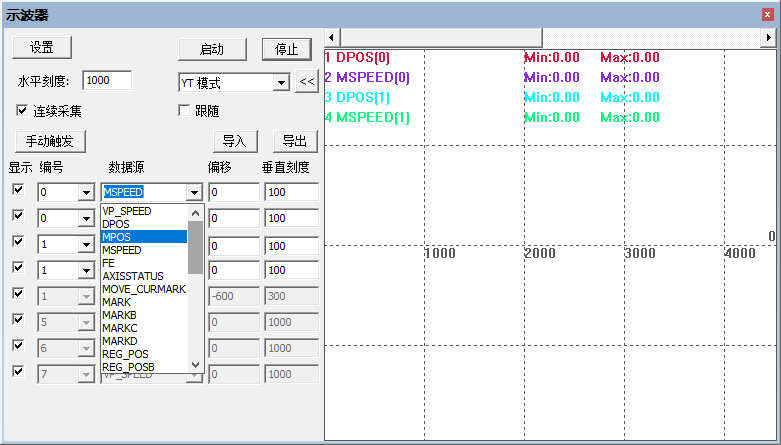
Data Source: Choose the type of data to be collected, as shown in the figure below, select from the drop-down menu, multiple types of parameters are available.

Offset: Setting for the vertical axis offset of the waveform.

Vertical Scale: The scale of one grid on the vertical axis.

⊙ To set oscilloscope parameters such as axis number, data source, and to open the oscilloscope settings window, you must stop the oscilloscope first before setting.

Click the “Settings” button on the main interface to pop up the “Oscilloscope Settings” window as shown below.

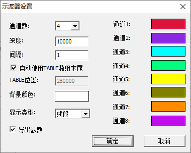
Number of Channels: Total number of data channels to be sampled, supporting up to 8 channels for simultaneous sampling.

Depth: Total number of sampling data points; the greater the depth, the more data points sampled; this data is invalid in continuous sampling mode.

Interval: Sampling time interval; this parameter refers to the system cycle SERVO_PERIOD, which is set to 1ms by default. Setting an interval of 1 means sampling once every 1ms. The system cycle is related to the controller firmware version. Generally, the smaller the interval, the more accurate the sampled data, and the greater the amount of data per unit time.

TABLE Position: Set the location where data is stored when not enabling continuous sampling; by default, it automatically uses the end space of TABLE data, but it can also be customized; however, care should be taken not to overlap with the TABLE data area used by the program. In continuous sampling mode, the sampled data is cached on the PC.

Background Color/Channel Color: Set the background color and the color corresponding to each channel waveform.

Display Type: Two curve types are available: points and line segments. Line segments fit the sampled points into a line, making it easier to identify abnormal data.

Export Parameters: When you need to export oscilloscope data, check before sampling, wait for sampling to finish, and then select export from the main interface.

Import: The oscilloscope must be in a stopped state to import data; successful import will reproduce the sampled waveform.

Method for Importing Sampling Data: Click “Import” and select the data file to be imported, which should be of the type previously exported from the oscilloscope, then open it.

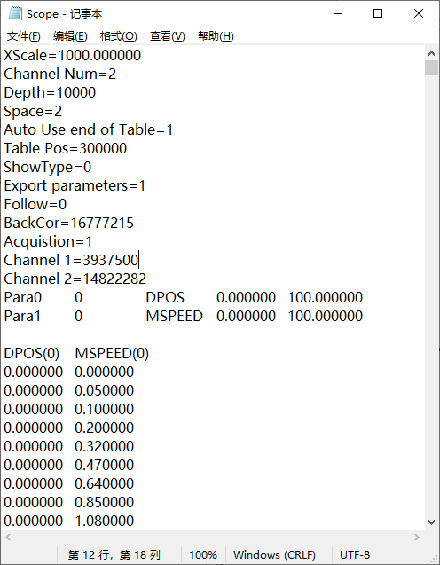
Export: Export parameters include oscilloscope parameter settings and the data types of each channel and each sampled data point.

Method for Exporting Sampling Data: First, check “Export Parameters” in the settings, start oscilloscope sampling, and after sampling is complete, click “Export” to choose a folder to save the oscilloscope data; the exported data will be in text file format.

As shown in the figure below, the exported data for sampled axis 0’s DPOS position and MSPEED speed from two channels.

3

Oscilloscope Sampling Method

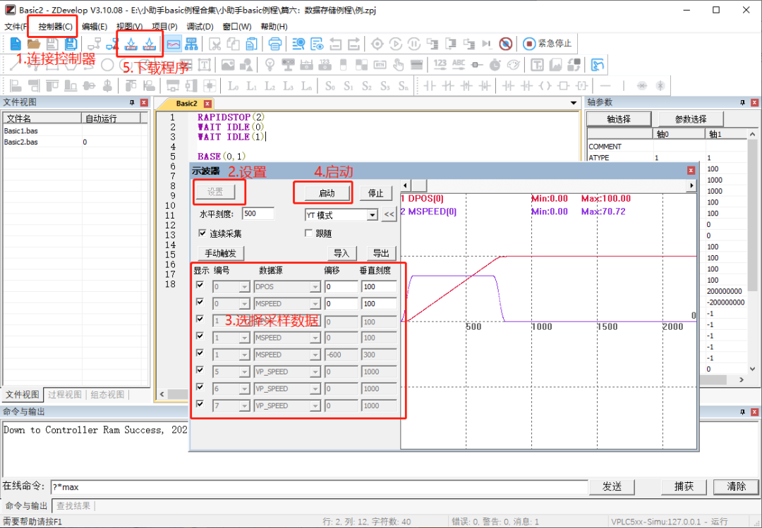
Step 1: Open the project, connect the controller or simulator, and then open the oscilloscope window(You must connect to the controller or simulator before operating the oscilloscope window).

Step 2: In the oscilloscope window, click “Settings”, select the number of sampling channels, sampling depth, sampling interval, and storage location for sampling data TABLE (Generally, automatically using the end space of the TABLE array is sufficient). After completing the settings, confirm and save the current settings.

Step 3: Then select the sampling data number and data source.

Step 4: After parameter settings are completed, click the “Start” button and wait for the trigger sampling.

Step 5: Download the program to the controller to run; the program must include the TRIGGER command to automatically trigger the oscilloscope sampling. At this time, the oscilloscope will start sampling and display the waveforms of different data sources. You can adjust the display scale and waveform offset to facilitate observation of different waveforms.

2. Precautions for Using the Oscilloscope

(1)Continuous Sampling Function

If continuous sampling is not selected, the oscilloscope will automatically stop sampling after reaching the sampling depth.

Check continuous sampling on the oscilloscope main interface, and after starting the oscilloscope, once the oscilloscope triggers sampling, it will continue to sample. Even after reaching the sampling depth, it will continue sampling, ignoring the set sampling depth, until the stop button is pressed.

All waveform sampling data from continuous sampling can be exported.

(2)XY Mode/XYZ Mode

Since these two sampling modes combine the data of the first two/three channels, attention should be paid to the types of data sources. Some data combinations are meaningless; for example, combining speed and position curves results in a meaningless composite curve, which is generally used to view the composite interpolation trajectory.

(3)Oscilloscope Sampling Time Calculation

For example: Depth: 10000, Interval: 5

In non-continuous sampling mode, if the system cycle SERVO_PERIOD=1000, which is a 1ms trajectory planning cycle, an interval of 5 means sampling one data point every 5ms, collecting a total of 10000 data points, resulting in a sampling time length of 50s.

The minimum sampling time interval is one system cycle; setting a smaller value is ineffective.

(4)Calculation of TABLE Data End Storage Space

In non-continuous sampling mode, the location for storing captured data can be set, generally defaulting to automatically use the end space of TABLE data, at which point the starting space address is automatically calculated based on the size of the sampled data.

Calculation Method: Size of sampled data = number of channels * depth

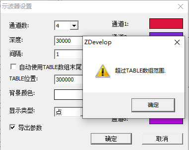
Example: If the size of the controller’s TABLE space is 320000, sampling 4 channels with a depth of 30000, each sample point occupies one TABLE, thus occupying 4*30000 = 120000 TABLE positions, resulting in 320000-120000=200000. The starting position of the TABLE at this time is 200000.

The data storage location can also be configured manually; if using the above channel number and depth, the starting TABLE space configured manually cannot exceed 200000, otherwise it cannot be set, as shown in the figure below.

4

Example of Oscilloscope Usage

1. Example of Linear Interpolation

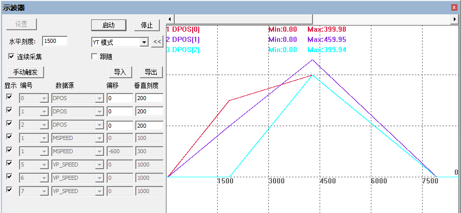
RAPIDSTOP(2)WAIT IDLE(0)WAIT IDLE(1)WAIT IDLE(2)BASE(0,1,2)        ' Axis selection, main axis is axis 0ATYPE=1,1,1        ' Set as pulse axis typeUNITS=100,100,100  ' Pulse equivalent settingsSPEED=100,10,1000  ' Only main axis speed 100 takes effect, serves as composite motion speedACCEL=1000,1000,1000DECEL=1000,1000,1000SRAMP=100,100,100DPOS=0,0,0TRIGGER            ' Automatically trigger oscilloscopeMOVE(300,200)      ' Axis 0, 1 linear interpolationMOVE(100,260,400)  ' Axis 0, 1, 2 linear interpolationMOVEABS(0,0,0)     ' Return to originEND

(1) DPOS position curve of three axes changing over time in YT mode

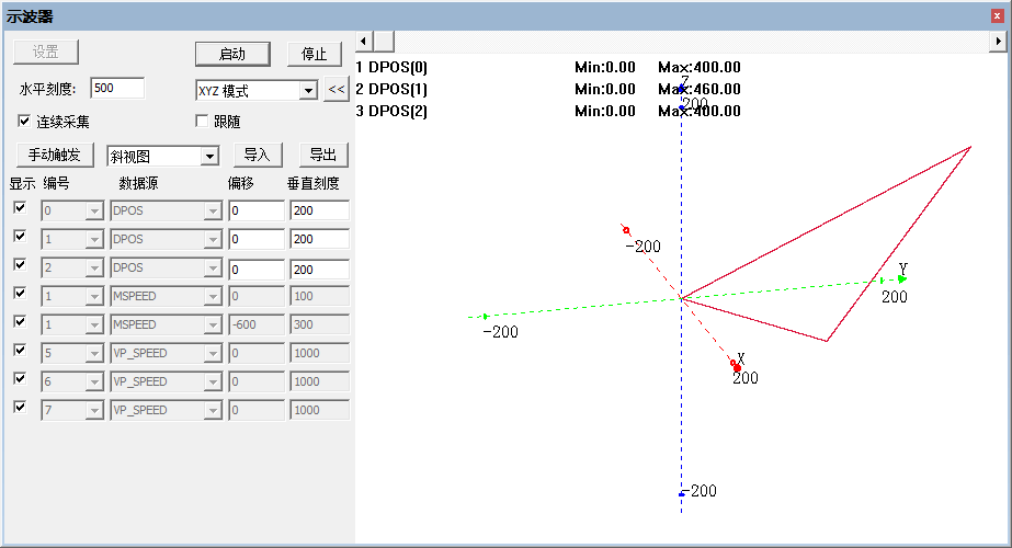
(2) Composite trajectory of three axes in XYZ mode, which is the actual processing trajectory

2. Example of Automatic Cam Flying Shear

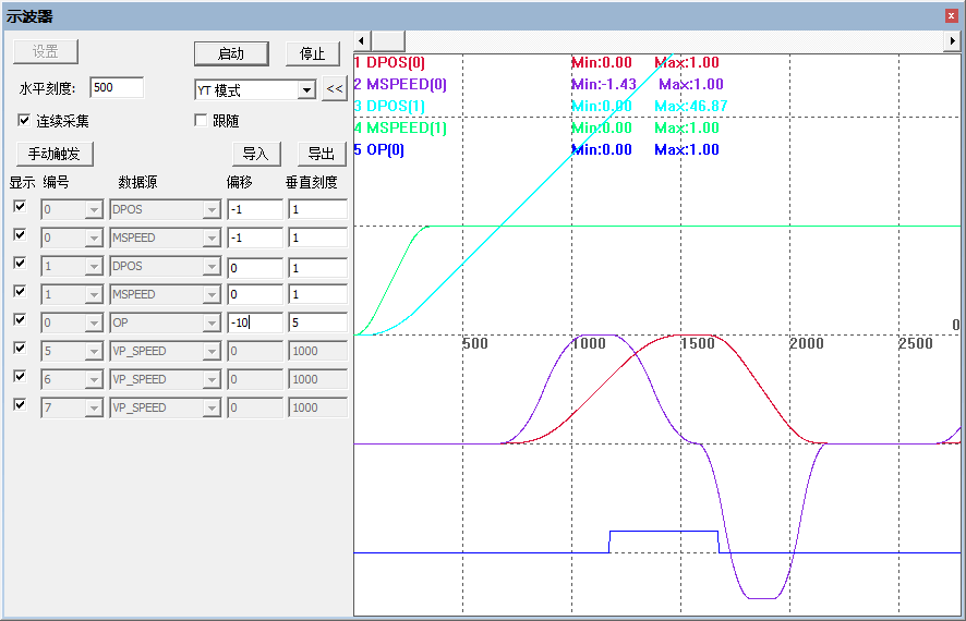
RAPIDSTOP(2)WAIT IDLE(0)WAIT IDLE(1)DATUM(0)BASE(0,1)UNITS=100000,100000ATYPE=1,1DPOS=0,0SPEED=1,1 ' Profile running speed 1m/s, 60m/minACCEL=2,2 DECEL=2,2SRAMP=200,200 OP(0,OFF)VMOVE(1) AXIS(1) ' Profile continues to moveTRIGGER ' Automatically trigger oscilloscopeWHILE 1    BASE(0)     MOVELINK(0,1,0,0,1,8) AXIS(0)        ' Profile moves 1m forward, workbench remains stationary    MOVELINK(0.4,0.8,0.8,0,1,8) AXIS(0)  ' Workbench acceleration stage    MOVELINK(0.2,0.2,0,0,1,8) AXIS(0)    ' Speed synchronization follow 0.2m    MOVE_OP2(0,on,1000)                  ' Tool cuts down, rises after 1s (time must be calculated well)    MOVELINK(0.4,0.8,0,0.8,1,8) AXIS(0)  ' Workbench deceleration stage    MOVELINK(-1,1.2,0.5,0.5,1,8) AXIS(0) ' Workbench returns to starting pointWENDEND

The waveform of speed and position is shown in the figure below: Axis 1 is the conveyor belt moving at a constant speed, and axis 0 is the follow-up cutting axis.

Distance traveled by the workbench (follow-up axis): 0.4 (acceleration stage) + 0.2 (synchronization follow) + 0.4 (deceleration stage) = 1m unit, then -1m return movement.

Distance traveled by the profile (reference axis): 1 + 0.8 + 0.2 + 0.8 + 1.2 = 4m unit, moving at a constant speed throughout.

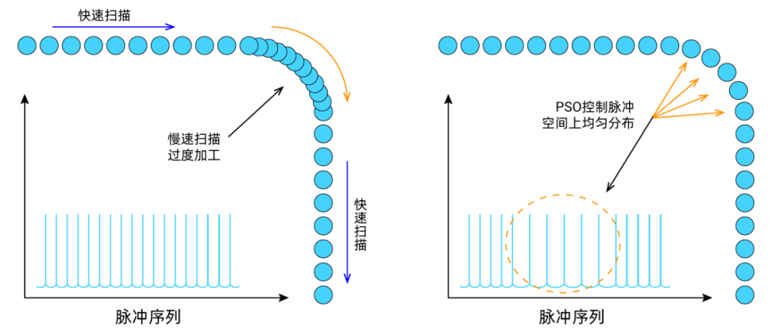
Hardware comparison output instruction trigger occurs after reaching the comparison point, outputting the OP signal. The PSO schematic diagram is shown in the figure below, demonstrated using ZMC432.

Position synchronous output schematic diagram

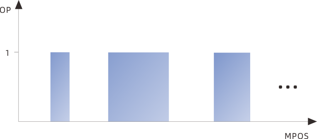
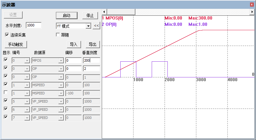
RAPIDSTOP(2)WAIT IDLE(0)BASE(0)DPOS=0MPOS=0ATYPE=1UNITS=100SPEED=100ACCEL=1000DECEL=1000OP(0,OFF)TABLE(0,50,100,150,200)        ' Comparison point coordinatesHW_PSWITCH2(2)                 ' Stop and delete unfinished comparison pointsHW_PSWITCH2(1, 0, 1, 0, 3,1)   ' Compare 4 points, operate output port 0TRIGGER                        ' Automatically trigger oscilloscope samplingMOVE(300)END

The waveform of output changing with trajectory is shown in the figure below. HW_PSWITCH2 controls the OP to reverse each time it reaches a TABLE point position; after all points are compared, OP will no longer reverse and will maintain the last level state.

4.2D or 3D PSO Output

Two-axis PSO position synchronous output, outputting the OP signal upon reaching comparison points, demonstrated using ZMC432.

The PSO function supports fixed cycle output and fixed distance output. As shown in the right figure, fixed distance output ensures that at corners where deceleration is needed, the output at the corner is also uniform and does not accumulate.

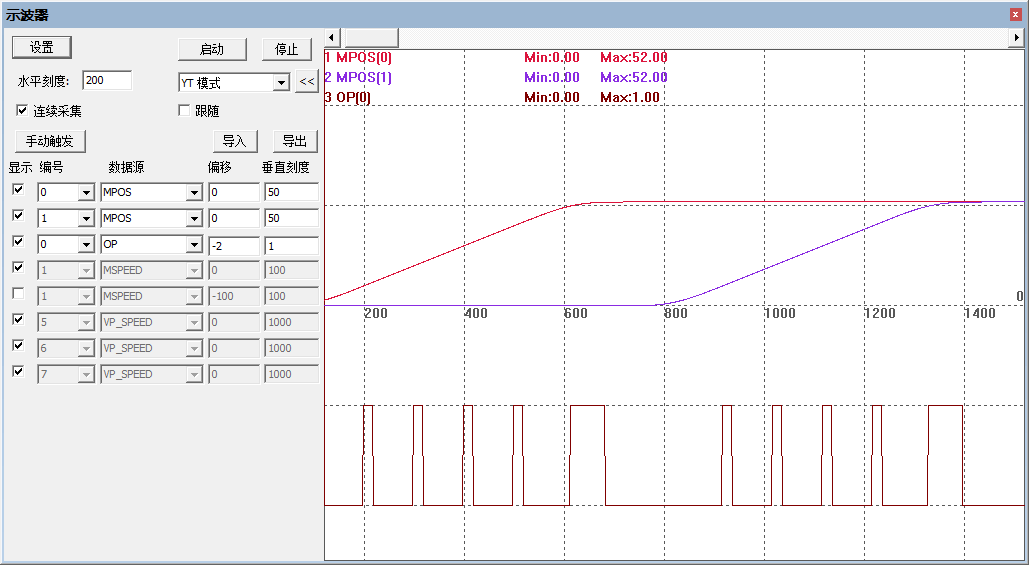
RAPIDSTOP(2)WAIT  IDLE(0)WAIT  IDLE(1)BASE(0,1)          ' Select XY axisATYPE=1,1          ' Pulse axis typeUNITS=100,100SPEED=100,100ACCEL=1000,1000DECEL=1000,1000SRAMP=100,100      ' S-curve speed smoothing' Set current position to 0,0DPOS=0,0MPOS=0,0' Pre-write position comparison points XY coordinates into table 10~49TABLE(10, 10,0,  12,0,  20,0,  22,0,  30,0)    ' table(10) starts writing 5 pointsTABLE(20, 32,0,  40,0,  42,0,  50,0,  52,0)    ' table(20) starts writing 5 pointsTABLE(30, 52,10, 52,12, 52,20, 52,22, 52,30)  ' table(30) starts writing 5 pointsTABLE(40, 52,32, 52,40, 52,42, 52,50, 52,52)  ' table(40) starts writing 5 pointsGLOBAL pointNum        ' Number of comparison points, as it is a two-dimensional mode with 20 points, 40 table data pointNum=20?' Compare pulse position, precise output'SYSTEM_ZSET=3      ' Enable precise output, can select system_zset or axis_zset parameterAXIS_ZSET=3,3      ' Corresponding bit1:1 MOVE_OP precise function, 0 MOVE_OP ordinary outputHW_PSWITCH2(2)     ' First clear all comparisonsHW_PSWITCH2(25,0,1,10,pointNum,10)    ' Write comparisons, mode 25, operate output port 0DELAY(10)TRIGGER      ' Start oscilloscopeMOVEABS(0,0) ' Start movementMOVEABS(52,0)MOVEABS(52,52)END

(1)Waveform in YT mode is shown in the figure below

Comparing 20 points, OP reverses once each time; the last part of each motion is extended due to the inclusion of SRAMP speed smoothing, resulting in longer motion time for the same distance, and the time interval for OP reversal is correspondingly extended.

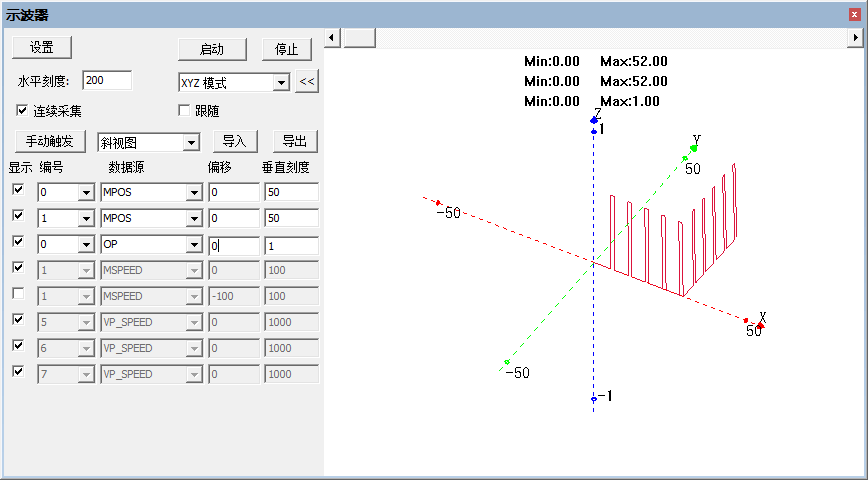
(2)3D waveform in XYZ mode is shown in the figure below

This concludes the sharing of the cost-effective EtherCAT motion controller (Part 9): using the oscilloscope.