Today, let’s explain what PID is through illustrations and text. What are the functions of each PID parameter? In what scenarios is PID used? Come and learn together!
What is PID?
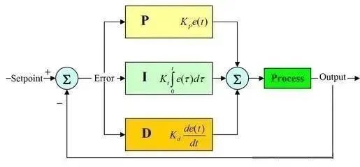
PID stands for “Proportional, Integral, Derivative,” and is a common control algorithm.
PID has a history of 107 years, and it’s not something mystical; everyone has seen actual applications of PID.
For example, in quadcopters, balancing cars… also in cruise control for cars, temperature controllers in 3D printers…
In situations where you need to keep a physical quantity “stable” (such as maintaining balance, stable temperature, speed, etc.), PID is very useful.
Now the question arises:
For instance, if I want to control a “rapid heater” to keep the temperature of a pot of water at 50°C, why do we need calculus theory for such a simple task?
You must be thinking:
Isn’t it simple? If it’s below 50 degrees, heat it up; if it’s above 50 degrees, cut the power. A few lines of code can be written in Arduino in no time.
That’s right! In cases where the requirements are not high, you can indeed do it this way. But! If we put it another way, you’ll see where the problem lies:
What if my control object is a car?
If I want the car’s speed to remain at 50 km/h, would you dare to do it this way?
Imagine, if the car’s cruise control computer detects that the speed is 45 km/h at a certain time. It immediately commands the engine: accelerate!
As a result, the engine suddenly goes to 100% throttle, and the car quickly accelerates to 60 km/h.
Then the computer issues a command: brake!
Result: screech……………wow…………(passengers throw up)
Therefore, in most cases, using “on-off” control for a physical quantity seems rather crude. Sometimes, it cannot maintain stability. Because microcontrollers and sensors are not infinitely fast, collecting and controlling takes time.
Moreover, the controlled object has inertia. For example, if you unplug a heater, its “residual heat” (i.e., thermal inertia) may still cause the water temperature to rise for a while.
Let’s first discuss the three basic parameters of the PID controller: kP, kI, kD.
The Role of kP:
P means proportional. Its effect is the most obvious, and its principle is the simplest. Let’s talk about it:
The quantity to be controlled, such as water temperature, has its current value and our expected target value.
-
When the two values are close, let the heater “gently” heat up.
-
If, for some reason, the temperature drops significantly, let the heater “apply some force” to heat up.
-
If the current temperature is much lower than the target temperature, let the heater “work at full power” to quickly bring the water temperature close to the target.
This is the role of P. Compared to the on-off control method, isn’t it much more “refined”?
When actually writing the program, just establish a linear relationship between the deviation (target minus current) and the “adjustment strength” of the control device, and you can achieve the most basic “proportional” control.
The larger kP is, the more aggressive the adjustment action. Reducing kP will make the adjustment action more conservative.
If you are making a balancing car, with the effect of P, you will find that the balancing car shakes back and forth around the balance angle, making it quite difficult to stabilize.
If you’ve reached this step—congratulations! You’re just a small step away from success!
The Role of kD:
D’s role is easier to understand, so let’s discuss D first and then I.
We just discussed the role of P. You might notice that P alone seems insufficient to keep the balancing car upright; the water temperature also fluctuates, making the entire system not particularly stable, always “jittering”.
Imagine a spring: now at the balance position. Pull it a bit and then let go. It will oscillate because of low resistance and may oscillate for a long time before stopping at the balance position.
Now imagine: if the system shown above is submerged in water, and you pull it a bit: in this case, the time taken to return to the balance position is much shorter.
We need a control action that causes the “rate of change” of the controlled physical quantity to tend towards zero, similar to a “damping” effect.
Because when close to the target, the control effect of P is relatively small. The closer you get to the target, the gentler the action of P becomes. Many internal or external factors can cause small fluctuations in the control quantity.
The role of D is to make the velocity of the physical quantity approach zero; whenever this quantity has a velocity, D applies force in the opposite direction, striving to stop this change.
The larger the kD parameter, the stronger the force applied in the opposite direction to stop the velocity.
If it’s a balancing car, with both P and D control actions, if the parameters are adjusted correctly, it should be able to stand upright—let’s cheer!
Wait, it seems like the PID trio has one more member. It looks like PD can stabilize the physical quantity, so why do we need I?
Because we have overlooked an important situation:
The Role of kI:
Let’s take hot water as an example. Suppose someone takes our heating device to a very cold place and starts heating water. It needs to reach 50°C.
Under the influence of P, the water temperature slowly rises. When it reaches 45°C, he realizes a bad thing: the cooling speed of the water equals the heating speed controlled by P.
What should we do?
-
P thinks: I’m already very close to the target; I just need to heat gently.
-
D thinks: heating and cooling are equal, and the temperature is stable; I don’t think I need to adjust anything.
As a result, the water temperature remains at 45°C forever and can never reach 50°C.
As a person, based on common sense, we know that we should further increase the heating power. But how much should we increase?
The methods devised by predecessor scientists are truly clever.
Set up an integral quantity. As long as there is a deviation, keep integrating (accumulating) it and reflect it in the adjustment strength.
This way, even if the difference between 45°C and 50°C is small, over time, as long as the target temperature is not reached, this integral quantity will keep increasing. The system will gradually realize: the target temperature has not been reached, and power should be increased!
Once the target temperature is reached, assuming the temperature remains stable, the integral value will no longer change. At this point, the heating power equals the cooling power. However, the temperature remains a steady 50°C.
The larger the kI value, the greater the coefficient multiplied during integration, and the more pronounced the integral effect.
Therefore, the role of I is to reduce the static error, keeping the controlled physical quantity as close to the target value as possible.
There is also a problem when using I: the integral limit needs to be set to prevent the integral quantity from becoming too large when initially heating, making it difficult to control.
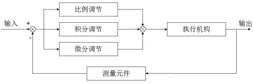
PID Control Principle:
1. Proportional (P) Control Proportional control is the simplest control method. The output of its controller is proportional to the input error signal. When only proportional control is used, the system output has a steady-state error.
2. Integral (I) Control In integral control, the output of the controller is proportional to the integral of the input error signal. For an automatic control system, if there is a steady-state error after reaching a steady state, this control system is said to have a steady-state error or is simply called a system with error. To eliminate steady-state error, an “integral term” must be introduced in the controller. The integral term depends on the time integral of the error, and as time increases, the integral term will increase. Thus, even if the error is small, the integral term will increase over time, pushing the output of the controller to further reduce the steady-state error until it equals zero. Therefore, the proportional + integral (PI) controller can keep the system free of steady-state error after reaching a steady state.
3. Derivative (D) Control In derivative control, the output of the controller is proportional to the derivative of the input error signal (i.e., the rate of change of the error). During the adjustment process of the automatic control system to overcome the error, oscillations or even instability may occur.
The reason is due to the presence of large inertia components (links) or lag components, which have a suppressing effect on the error, and their changes always lag behind the changes in the error.
The solution is to make the change of the error suppression effect “lead,” meaning that when the error approaches zero, the suppression effect should also be zero. This indicates that simply introducing the “proportional” term in the controller is often insufficient; the role of the proportional term is only to amplify the magnitude of the error, while the current need is to increase the “derivative” term, which can predict the trend of error changes.
Thus, a controller with proportional + derivative can make the error suppression control action equal to zero in advance, or even negative, thereby avoiding severe overshoot of the controlled quantity. Therefore, for controlled objects with large inertia or lag, a proportional + derivative (PD) controller can improve the dynamic characteristics of the system during the adjustment process.
General Methods for Tuning PID Controller Parameters:
Tuning the parameters of the PID controller is the core content of control system design. It determines the sizes of the proportional coefficient, integral time, and derivative time of the PID controller based on the characteristics of the controlled process. There are many methods for tuning PID controller parameters, which can be broadly classified into two categories:
Theoretical Calculation Tuning Method
This method primarily relies on the mathematical model of the system to theoretically calculate the controller parameters. The calculated data obtained from this method may not be directly usable and must be adjusted and modified through engineering practice;
Engineering Tuning Method
This method mainly relies on engineering experience, directly conducting tests in the control system, and is simple and easy to master, widely used in engineering practice. The engineering tuning methods for PID controller parameters mainly include critical ratio method, reaction curve method, and decay method.
Each of these methods has its characteristics, but their common point is that they all require experimentation and then adjust the controller parameters according to engineering experience formulas. However, regardless of which method is used to obtain the controller parameters, final adjustments and improvements must be made during actual operation.
Currently, the critical ratio method is commonly used. The steps for tuning PID controller parameters using this method are as follows:
-
First, preselect a sufficiently short sampling period to allow the system to operate;
-
Only add the proportional control element until the system exhibits critical oscillation in response to a step input; record the proportional gain and the period of critical oscillation at this time;
-
Calculate the PID controller parameters using formulas under certain control degrees.
The setting of PID parameters is based on experience and familiarity with the process, tracking the measured values against the set value curve to adjust the sizes of P, I, and D.
Common Mnemonics:
Find the best parameter tuning, check in order from small to large;
First is proportional, then integral, finally add derivative;
If the curve oscillates frequently, increase the proportional dial;
If the curve drifts around the bay, decrease the proportional dial;
If the curve deviates and returns slowly, decrease the integral time;
If the curve fluctuates for a long period, increase the integral time;
If the curve oscillates rapidly, first reduce the derivative;
If the dynamic difference is large and the fluctuation is slow, increase the derivative time;
Ideal curve has two waves, high in front and low behind, ratio 4:1;
By looking, adjusting, and analyzing more, the quality of regulation will not be low.
Personally, I believe the size of PID parameters should depend on the specific situation of the controlled object; on the other hand, it is based on experience. P solves amplitude oscillation; a large P will lead to a larger amplitude of oscillation but a smaller oscillation frequency, resulting in a longer stabilization time for the system; I solves the speed of action response; a large I will slow down the response speed, and vice versa; D eliminates static errors, and generally D is set smaller and has a smaller impact on the system.
How to Best Adjust PID Parameters:
(1) Tuning the proportional control: Increase the proportional control action from small to large, observing each response until a quick reaction with minimal overshoot is achieved.
(2) Tuning the integral element: If the steady-state error cannot be met under proportional control, integral control needs to be added. First, reduce the proportional coefficient selected in step (1) to 50-80% of its original value, then set the integral time to a larger value and observe the response curve. Then reduce the integral time, increase the integral effect, and adjust the proportional coefficient accordingly, repeating until a satisfactory response is achieved, determining the parameters for proportional and integral.
(3) Tuning the derivative element: If after step (2), PI control can only eliminate steady-state error, but the dynamic process is unsatisfactory, then derivative control should be added to form PID control. Set the derivative time TD=0, gradually increase TD while correspondingly changing the proportional coefficient and integral time, repeating until satisfactory control effects and PID control parameters are obtained.
Animated Demonstration
First, watch the animation to learn about PID:
The initial state of the system is 0, and the target state is 10.
Let’s first show the process of traversing parameters.
The following animations demonstrate the effects of each parameter:

In practical engineering, the most widely used regulation control law is proportional, integral, derivative control, abbreviated as PID control, also known as PID regulation. Since its introduction nearly 70 years ago, the PID controller has become one of the main technologies in industrial control due to its simple structure, good stability, reliable operation, and ease of adjustment.
PID regulation control is a traditional control method suitable for temperature, pressure, flow, liquid level, and almost all fields. In different fields, only the PID parameters need to be set differently. As long as the parameters are set correctly, good results can be achieved, reaching control requirements of 0.1% or even higher.
The Story of PID
Little Ming received a task: there is a water tank that leaks (and the leak rate is not necessarily constant), requiring the water level to be maintained at a certain position. Once the water level is found to be lower than the required position, water must be added to the tank.
After receiving the task, Little Ming stayed by the tank, and after a long time, he felt bored, so he went inside to read a novel, checking the water level every 30 minutes.
The water leaked too quickly, and every time Little Ming checked, the water was almost gone, far from the required height. Little Ming changed to check every 3 minutes, but then each time he came, the water hadn’t leaked much, and he didn’t need to add water; coming too frequently was useless work.
After several experiments, he determined to check every 10 minutes. This checking time is called the sampling period.
At first, Little Ming used a ladle to add water, but the faucet was more than ten meters away from the tank, requiring several trips to add enough water. So Little Ming switched to using a bucket, adding one bucket at a time, which reduced the number of trips but overflowed the tank several times, accidentally wetting his shoes. Little Ming thought again: I won’t use a ladle or a bucket; I’ll use a basin. After a few tries, he found it just right, not needing too many trips and not letting the water overflow. The size of this water-adding tool is called the proportional coefficient.
Little Ming also noticed that although the water would not overflow, it sometimes would exceed the required position significantly, still risking wet shoes.
He then thought of a way to install a funnel on the water tank, adding water not directly into the tank but into the funnel to let it add slowly. This solved the overflow problem, but the water-adding speed became slow, sometimes not keeping up with the leak rate.
So he tried different sizes of funnels to control the water-adding speed and finally found a satisfactory funnel. The time taken for the funnel is called the integral time.
Little Ming finally breathed a sigh of relief, but suddenly the task requirements became stricter; the timeliness of controlling the water level was greatly increased. Once the water level drops too low, it must be immediately raised to the required position, without exceeding too much; otherwise, he wouldn’t get paid. Little Ming was in trouble again!
He thought hard again and finally came up with a solution: keep a basin of standby water nearby. As soon as he noticed the water level was low, he would add a basin of water without going through the funnel, ensuring timeliness, but the water level sometimes would rise too high.
He then drilled a hole slightly above the required water level and connected a pipe to a lower standby bucket, allowing the excess water to drain out through the hole. The speed of this water draining out is called the derivative time.
Seeing several posts asking about sampling periods, I came up with this story on the spot. The analogy of the derivative is a bit forced, but if it helps understanding, it’s worth it. This is a beginner-level explanation, and if it helps newbies understand PID, I am satisfied.
In the story, Little Ming’s experiments were done independently step by step, but in reality, the water-adding tool, funnel diameter, and overflow hole size would all simultaneously affect the water-adding speed and the size of the water level overshoot. After conducting later experiments, adjustments often need to be made to the results of earlier experiments.
Little Ming’s experiments were conducted independently step by step, but in practice, the water-adding tool, funnel diameter, and overflow hole size would all simultaneously affect the water-adding speed and the size of the water level overshoot. After conducting later experiments, adjustments often need to be made to the results of earlier experiments.
Using PID control, a person pours half a cup of water into a cup marked with a scale and then stops;
-
Set point: the half-cup mark on the cup;
-
Actual value: the actual water amount in the cup;
-
Output value: the amount of water poured from the kettle and the amount of water scooped from the cup;
-
Measurement: the person’s eyes (equivalent to a sensor)
-
Execution object: the person
-
Positive execution: pouring water
-
Negative execution: scooping water
(1) P Proportional Control
Meaning that when the water level in the cup does not reach the half-cup mark, the person pours a certain amount of water from the kettle into the cup; if the water exceeds the mark, a certain amount is scooped out. This action might result in stopping before reaching the half-cup or overflowing.
Explanation: P proportional control is the simplest control method. Its controller output is proportional to the input error signal. When only proportional control is used, there is a steady-state error in the system output (Steady-state error).
(2) PI Integral Control
Meaning that a certain amount of water is poured into the cup, and if the water level does not meet the mark, it continues to pour. If the water exceeds half a cup, it scoops water out, repeating until the water level reaches the mark.
Explanation: In integral control, the output of the controller is proportional to the integral of the input error signal. For an automatic control system, if there is a steady-state error after reaching a steady state, this control system is said to have a steady-state error or is simply called a system with steady-state error (System with Steady-state Error). To eliminate steady-state error, an “integral term” must be introduced in the controller. The integral term depends on the time integral of the error, and as time increases, the integral term will increase. Thus, even if the error is small, the integral term will increase over time, pushing the output of the controller to further reduce the steady-state error until it equals zero. Therefore, the proportional + integral (PI) controller can keep the system free of steady-state error after reaching a steady state.
(3) PID Derivative Control
Meaning that the person looks at the distance between the water level in the cup and the mark. When the difference is large, they pour a large amount of water; when they see the water level approaching the mark, they reduce the amount poured, slowly approaching the mark until stopping at the marked position.
If they can stop precisely at the mark, it is no static error control; if they stop near the mark, it is static error control.
Explanation: In derivative control, the output of the controller is proportional to the derivative of the input error signal (i.e., the rate of change of the error). In practical engineering, the most widely used regulation control law is proportional, integral, and derivative control, abbreviated as PID control, also known as PID regulation.
Since the introduction of the PID controller nearly 70 years ago, it has become one of the main technologies in industrial control due to its simple structure, good stability, reliable operation, and ease of adjustment.
When the structure and parameters of the controlled object cannot be fully mastered, or precise mathematical models cannot be obtained, and other control theory techniques are difficult to apply, the structure and parameters of the system controller must rely on experience and on-site debugging. In this case, applying PID control technology is the most convenient.
That is, when we do not fully understand a system and the controlled object or cannot obtain system parameters through effective measurement means, PID control technology is the most suitable. PID control can also be PI and PD control.
The PID controller calculates the control quantity based on the system error using proportional, integral, and derivative calculations.
PID Parameters
1. Proportional (P) Control
Proportional control is the simplest control method. Its controller output is proportional to the input error signal. When only proportional control is used, the system output has a steady-state error (Steady-state error).
2. Integral (I) Control
In integral control, the output of the controller is proportional to the integral of the input error signal. For an automatic control system, if there is a steady-state error after reaching a steady state, this control system is said to have a steady-state error or is simply called a system with steady-state error (System with Steady-state Error). To eliminate steady-state error, an “integral term” must be introduced in the controller. The integral term depends on the time integral of the error, and as time increases, the integral term will increase. Thus, even if the error is small, the integral term will increase over time, pushing the output of the controller to further reduce the steady-state error until it equals zero. Therefore, the proportional + integral (PI) controller can keep the system free of steady-state error after reaching a steady state.
3. Derivative (D) Control
In derivative control, the output of the controller is proportional to the derivative of the input error signal (i.e., the rate of change of the error). During the adjustment process of the automatic control system to overcome the error, oscillations or even instability may occur.
The reason is due to the presence of large inertia components (links) or lag components, which have a suppressing effect on the error, and their changes always lag behind the changes in the error. The solution is to make the change of the error suppression effect “lead,” meaning that when the error approaches zero, the suppression effect should also be zero.
This indicates that simply introducing the “proportional” term in the controller is often insufficient; the role of the proportional term is only to amplify the magnitude of the error, while the current need is to increase the “derivative” term, which can predict the trend of error changes. Thus, a controller with proportional + derivative can make the error suppression control action equal to zero in advance, or even negative, thereby avoiding severe overshoot of the controlled quantity. Therefore, for controlled objects with large inertia or lag, a proportional + derivative (PD) controller can improve the dynamic characteristics of the system during the adjustment process.
When tuning PID parameters, if it is possible to theoretically determine the PID parameters, that is the ideal method; however, in practical applications, more often, the parameters of PID are determined through trial and error.
Increasing the proportional coefficient P generally speeds up the system’s response, which is beneficial for reducing static error in the presence of static error; however, an excessively large proportional coefficient can lead to significant overshoot and oscillation, reducing stability.
Increasing the integral time I helps reduce overshoot and oscillation, increasing the system’s stability; however, it prolongs the time to eliminate static error.
Increasing the derivative time D helps speed up the system’s response, reducing the overshoot and increasing stability, but weakens the system’s ability to suppress disturbances.
During trial and error, you can refer to the effects of the above parameters on the system control process and implement the tuning steps of first proportional, then integral, and finally derivative.
Methods for Tuning PID Controller Parameters
Tuning the parameters of the PID controller is the core content of control system design. It determines the sizes of the proportional coefficient, integral time, and derivative time of the PID controller based on the characteristics of the controlled process. There are many methods for tuning PID controller parameters, which can be broadly classified into two categories:
1. Theoretical Calculation Tuning Method
This method primarily relies on the mathematical model of the system to theoretically calculate the controller parameters. The calculated data obtained from this method may not be directly usable and must be adjusted and modified through engineering practice;
2. Engineering Tuning Method
This method mainly relies on engineering experience, directly conducting tests in the control system, and is simple and easy to master, widely used in engineering practice. The engineering tuning methods for PID controller parameters mainly include critical ratio method, reaction curve method, and decay method.
Each of these methods has its characteristics, but their common point is that they all require experimentation and then adjust the controller parameters according to engineering experience formulas. However, regardless of which method is used to obtain the controller parameters, final adjustments and improvements must be made during actual operation.
Currently, the critical ratio method is commonly used. The steps for tuning PID controller parameters using this method are as follows:
-
First, preselect a sufficiently short sampling period to allow the system to operate;
-
Only add the proportional control element until the system exhibits critical oscillation in response to a step input; record the proportional gain and the period of critical oscillation at this time;
-
Calculate the PID controller parameters using formulas under certain control degrees.
The setting of PID parameters is based on experience and familiarity with the process, tracking the measured values against the set value curve to adjust the sizes of P, I, and D.
Common Mnemonics:
Find the best parameter tuning, check in order from small to large;
First is proportional, then integral, finally add derivative;
If the curve oscillates frequently, increase the proportional dial;
If the curve drifts around the bay, decrease the proportional dial;
If the curve deviates and returns slowly, decrease the integral time;
If the curve fluctuates for a long period, increase the integral time;
If the curve oscillates rapidly, first reduce the derivative;
If the dynamic difference is large and the fluctuation is slow, increase the derivative time;
Ideal curve has two waves, high in front and low behind, ratio 4:1;
By looking, adjusting, and analyzing more, the quality of regulation will not be low.
Personally, I believe the size of PID parameters should depend on the specific situation of the controlled object; on the other hand, it is based on experience. P solves amplitude oscillation; a large P will lead to a larger amplitude of oscillation but a smaller oscillation frequency, resulting in a longer stabilization time for the system; I solves the speed of action response; a large I will slow down the response speed, and vice versa; D eliminates static errors, and generally D is set smaller and has a smaller impact on the system.
How to Best Adjust PID Parameters:
(1) Tuning the proportional control: Increase the proportional control action from small to large, observing each response until a quick reaction with minimal overshoot is achieved.
(2) Tuning the integral element: If the steady-state error cannot be met under proportional control, integral control needs to be added. First, reduce the proportional coefficient selected in step (1) to 50-80% of its original value, then set the integral time to a larger value and observe the response curve. Then reduce the integral time, increase the integral effect, and adjust the proportional coefficient accordingly, repeating until a satisfactory response is achieved, determining the parameters for proportional and integral.
(3) Tuning the derivative element: If after step (2), PI control can only eliminate steady-state error, but the dynamic process is unsatisfactory, then derivative control should be added to form PID control. Set the derivative time TD=0, gradually increase TD while correspondingly changing the proportional coefficient and integral time, repeating until satisfactory control effects and PID control parameters are obtained.
PID’s 15 Basic Concepts
Without the right tools, don’t take on delicate tasks. To master and apply PID effectively, it is essential to learn the basic concepts to equip ourselves, some concepts will be paired with commonly used representations in practical engineering, starting with “Actual: “
1. Controlled Quantity Reflects the actual fluctuation of the controlled object. The controlled quantity is frequently changing.
Actual: Commonly detected feedback values, such as yout(t).
2. Set Point The set point of the PID regulator is the value that people expect the controlled quantity to reach. The set point can be fixed or variable.
Actual: Manually set, often represented as rin(t).
3. Control Output The control output of the PID regulator is the directive issued to the external execution structure based on the changes in the controlled quantity, i.e., the output of the entire regulator. Note the distinction from the controlled quantity yout(t); these two are entirely different concepts and are often confused.
Actual: The formula you often see “u(t)=kp[e(t)+1/TI∫e(t)dt+TD*de(t)/dt]” contains u(t).
4. Input Deviation The input deviation is the difference between the controlled quantity and the set point.
Actual: error(t)=rin(t)-yout(t).
5. P (Proportional) P represents the proportional action, simply put, it is the input deviation multiplied by a coefficient.
Actual: For example, kp, KP are the same.
6. I (Integral) I represents the integral, simply put, it is the integral operation of the input deviation.
7. D (Derivative) D represents the derivative, simply put, it is the derivative operation of the input deviation.
8. Basic PID Formula The tuning process of PID regulator parameters can be simply described as first setting the system to pure proportional action, gradually increasing the proportional action to produce equal amplitude oscillations, recording the proportional action and oscillation period, then multiplying this proportional action by 0.6 and extending the integral action appropriately.
KP= 0.6	ext{*}Km

KD= KP	ext{*}rac{	ext{π}}{4ω} 	ext{ or } KD= KP	ext{*}rac{tu}{8}

KI= KP	ext{*}rac{ω}{	ext{π}} 	ext{ or } KI= rac{2KP}{tu}

KP: Proportional control parameter;

KD: Integral control parameter;

KI: Derivative control parameter;
Km: The proportional value at which the system begins to oscillate, commonly referred to as the critical proportional value;
ω: The frequency during equal amplitude oscillations, where tu is the oscillation period. Here tuω =2π, not tuω=1. Those who have studied Fourier and Laplace transforms should understand why this is the case; we will not delve into it here.
9. Single Loop A single loop is a control system with only one PID regulator.
10. Cascade When one PID is not enough, cascade means connecting two PIDs in series to form a cascade control system, also known as a dual-loop control system. In a cascade control system, there are primary and secondary controls.
In a cascade control system, the PID that regulates the controlled quantity is called the primary control, while the PID that directly commands the actuator is called the secondary control. The output of the primary control enters the secondary control as the set point for the secondary control. The primary control uses a single-loop PID regulator, while the secondary control uses an externally specified regulator.
11. Positive Action
For the PID regulator, when the control output increases with the increase of the controlled quantity and decreases with the decrease of the controlled quantity, it is called PID positive action.
12. Negative Action
For the PID regulator, when the control output decreases with the increase of the controlled quantity and increases with the decrease of the controlled quantity, it is called PID negative action.
13. Dynamic Deviation
During the regulation process, the deviation between the controlled quantity and the set point changes at any time; the deviation between the two at any moment is called dynamic deviation.
14. Static Deviation
After the regulation stabilizes, the remaining deviation between the controlled quantity and the set point is called static deviation. Eliminating static deviation is achieved through the integral action of the PID regulator.
15. Feedback
The display of the regulator’s adjustment action causes the controlled quantity to start changing from rising to falling or from falling to rising is called feedback.


Disclaimer: This article is a network reprint, and the copyright belongs to the original author. If there are any copyright issues with the videos, images, or text used in this article, please leave a message at the end of the article, and we will handle it as soon as possible! The content of this article reflects the views of the original author and does not represent the views of this public account or its authenticity.


Recommended Reading

Add WeChat and reply “Join Group“
We will add you to the technical exchange group!
Domestic Chips | Automotive Electronics | Internet of Things | New Energy | Power Supply | Industrial | Embedded…..
Reply with any content you want to search for in the public account, such as keywords, technical terms, bug codes, etc., and you will easily get feedback on professional technical content related to it. Go try it!
If you want to see our articles regularly, you can go to our homepage, click the three small dots in the upper right corner, and select “Set as Starred”.
Welcome to scan and follow us