Learning PID Control Through Stories and Animations

Part One

The initial state of the system is 0, and the target state is 10.

Let’s first demonstrate the process of traversing parameters.

The following animations show the effects of each parameter:

Part Two

Little Ming received a task:

There is a water tank leaking (and the leak rate may not be constant), and the water level must be maintained at a certain position. Once the water level is found to be lower than the required position, water must be added to the tank.

After receiving the task, Little Ming kept watching the water tank. After a long time, he felt bored and ran into the room to read a novel, checking the water level every 30 minutes. The water leaked too quickly, and every time Little Ming checked, the water was almost gone, far from the required height. Little Ming changed to checking every 3 minutes, but found that the water hardly leaked, so he didn’t need to add water. Checking too frequently was a waste of effort. After several experiments, he decided to check every 10 minutes. This checking time is called the sampling period.

At first, Little Ming used a ladle to add water, but the faucet was more than ten meters away from the tank, and he often had to run several times to add enough water. So Little Ming switched to using a bucket, which allowed him to add a whole bucket at a time, reducing the number of trips and speeding up the water addition. However, he overflowed the tank several times and accidentally got his shoes wet. Little Ming then thought, I won’t use a ladle or a bucket; I’ll use a basin. After a few tries, he found it was just right, not needing to run too many times and not overflowing. The size of this water addition tool is called the proportional coefficient.

Little Ming also found that while he wouldn’t overflow, sometimes the water would be much higher than the required position, still risking wet shoes. He thought of a way to install a funnel on the tank, so that every time he added water, it wouldn’t go directly into the tank but would go into the funnel to be added slowly. This solved the overflow problem, but the water addition speed became slow, sometimes unable to keep up with the leak rate. So he tried different sizes of funnels to control the water addition speed and finally found a satisfactory funnel. The time for the funnel is called the integral time.

Little Ming finally breathed a sigh of relief, but the task requirements suddenly tightened. The timeliness of controlling the water level was greatly increased. Once the water level was too low, water must be added to the required position immediately, and it must not exceed too much, or he wouldn’t get paid. Little Ming was troubled again! So he thought hard and finally came up with a solution: keep a basin of spare water nearby. As soon as he found the water level low, he would pour a basin of water in without going through the funnel, ensuring timeliness, but sometimes the water level would be too high. He then drilled a hole just above the required water level and connected a pipe to the spare bucket below, allowing the excess water to leak out from the upper hole. The speed at which the water leaks out is called the differential time.

I got this story after seeing several articles about sampling periods. The analogy of differentiation is somewhat forced, but it helps with understanding.

For beginners, if it can help new users understand PID, that’s enough. In the story, Little Ming’s experiments are done independently step by step, but in reality, the water addition tools, funnel diameters, and overflow hole sizes all affect the water addition speed, and the magnitude of water level overshoot. After later experiments, it often requires modifying the results of previous experiments.

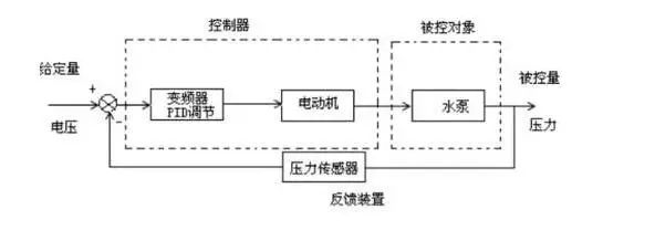
II. Control Model:

People use PID control to pour half a cup of water (marked with a scale) from a kettle into a cup, then stop;

Setpoint: The half-cup scale of the cup;

Actual value: The actual water volume in the cup;

Output value: The amount poured from the kettle and the amount scooped from the cup;

Measurement sensor: Human eyes

Execution object: Human

Positive execution: Pouring water

Negative execution: Scooping water

1. P Proportional Control, means that when a person sees that the water volume in the cup does not reach the half-cup scale, they pour a certain amount from the kettle into the cup, or if the water volume exceeds the scale, they scoop a certain amount out of the cup. This action may cause the cup to be less than half full or more than half full, and then stop.

Explanation: P proportional control is the simplest control method. The output of its controller is proportional to the input error signal. When only proportional control is used, the system output has a steady-state error (Steady-state error).

2. PI Integral Control, means pouring a certain amount into the cup. If the water volume is not at the scale, keep pouring. Later, if the water volume exceeds half a cup, scoop water out of the cup, and repeat until the water volume reaches the scale.

Explanation: In integral I control, the output of the controller is proportional to the integral of the input error signal. For an automatic control system, if there is a steady-state error after entering steady-state, this control system is said to have a steady-state error or is referred to as a system with steady-state error (System with Steady-state Error). To eliminate steady-state error, an “integral term” must be introduced into the controller. The integral term depends on the time integral of the error, and as time increases, the integral term will increase. Thus, even if the error is small, the integral term will increase over time, pushing the controller’s output to increase, further reducing the steady-state error until it equals zero. Therefore, the proportional + integral (PI) controller can ensure that the system has no steady-state error after entering steady-state.

3. PID Differential Control, means that when a person looks at the distance between the water volume and the scale, when the gap is large, they pour a large amount of water from the kettle. When they see that the water volume is about to approach the scale, they reduce the output amount from the kettle, slowly approaching the scale until stopping at the scale position. If it can finally stop precisely at the scale position, it is no steady-state error control; if it stops near the scale, it is steady-state error control.

Explanation: In differential control D, the output of the controller is proportional to the derivative of the input error signal (i.e., the rate of change of the error).

In engineering practice, the most widely used control regulation is proportional, integral, and differential control, collectively referred to as PID control, also known as PID regulation. The PID controller has been in existence for nearly 70 years, and due to its simple structure, good stability, reliable operation, and easy adjustment, it has become one of the main technologies in industrial control. When the structure and parameters of the controlled object cannot be fully grasped or an accurate mathematical model cannot be obtained, and other control theory techniques are difficult to apply, the structure and parameters of the system controller must be determined based on experience and field debugging. In such cases, PID control technology is the most convenient to use. That is, when we do not fully understand a system and the controlled object or cannot obtain system parameters through effective measurement methods, PID control technology is the most suitable. PID control also includes PI and PD control. The PID controller calculates the control quantity based on the system error using proportional, integral, and differential approaches.

Proportional (P) Control

Proportional control is the simplest control method. Its controller output is proportional to the input error signal. When only proportional control is used, the system output has a steady-state error (Steady-state error).

Integral (I) Control

In integral control, the output of the controller is proportional to the integral of the input error signal. For an automatic control system, if there is a steady-state error after entering steady-state, this control system is said to have a steady-state error or is referred to as a system with steady-state error (System with Steady-state Error). To eliminate steady-state error, an “integral term” must be introduced into the controller. The integral term depends on the time integral of the error, and as time increases, the integral term will increase. Thus, even if the error is small, the integral term will increase over time, pushing the controller’s output to increase, further reducing the steady-state error until it equals zero. Therefore, the proportional + integral (PI) controller can ensure that the system has no steady-state error after entering steady-state.

Differential (D) Control

In differential control, the output of the controller is proportional to the derivative of the input error signal (i.e., the rate of change of the error). In the process of regulating the automatic control system to overcome errors, oscillations or even instability may occur. This is caused by the presence of large inertia components (links) or delay components that suppress the error, whose changes always lag behind the changes in the error. The solution is to make the changes in the error suppression action “advance,” that is, when the error approaches zero, the error suppression action should be zero. This means that simply introducing a “proportional” term in the controller is often not enough; the proportional term only amplifies the magnitude of the error, while what is needed now is to add a “differential term,” which can predict the trend of error changes. Thus, a controller with proportional + differential can make the suppression of the error control action equal to zero in advance, or even negative, thereby avoiding serious overshoot of the controlled quantity. Therefore, for controlled objects with large inertia or delay, a proportional + differential (PD) controller can improve the dynamic characteristics of the system during the regulation process.

When tuning PID parameters, having a theoretical method to determine PID parameters is certainly the ideal method, but in practical applications, more often the PID parameters are determined through trial and error.

Increasing the proportional coefficient P generally speeds up the system’s response, which helps reduce static error in cases with static error, but too large a proportional coefficient may cause significant overshoot and oscillation, degrading stability.

Increasing the integral time I helps reduce overshoot, decrease oscillation, and increase system stability, but it extends the time to eliminate static error.

Increasing the differential time D helps speed up the system’s response and reduce overshoot, increasing stability, but it weakens the system’s ability to suppress disturbances.

During testing, the above parameters can be referenced for their influence on the system control process, and the adjustment of parameters should follow the tuning steps of first proportional, then integral, and finally differential.

General Methods for Tuning PID Controller Parameters:

Tuning PID controller parameters is the core content of control system design. It determines the size of the proportional coefficient, integral time, and differential time of the PID controller based on the characteristics of the controlled process. There are many methods for tuning PID controller parameters, which can be summarized into two main categories:

One is theoretical calculation tuning method. It mainly relies on the mathematical model of the system, determining the controller parameters through theoretical calculations. The calculated data obtained by this method may not be directly usable and must be adjusted and modified through engineering practice;

Two is engineering tuning method, which mainly relies on engineering experience, conducted directly in the control system experiments, and is widely used in engineering practice due to its simplicity and ease of mastery. The engineering tuning methods for PID controller parameters mainly include the critical proportional method, reaction curve method, and attenuation method. Each of these three methods has its characteristics, but they all share the common point of tuning controller parameters through experiments and according to engineering experience formulas. However, regardless of which method is used to obtain the controller parameters, final adjustments and improvements must be made during actual operation.

Currently, the critical proportional method is generally adopted. The steps for tuning PID controller parameters using this method are as follows:(1) First, pre-select a sufficiently short sampling period for the system to work; (2) Only add the proportional control link until the system’s step response exhibits critical oscillation, recording the proportional gain and critical oscillation period at this time; (3) Calculate the PID controller parameters through formulas under certain control degrees.

Setting PID parameters: relies on experience and familiarity with the process, tracking the measurement values against the set value curve, and adjusting P, I, and D accordingly.

Common Mnemonics in Books:

Find the best parameters by tuning from small to large;

First is proportional, then integral, and finally add differential;

If the curve oscillates frequently, increase the proportional dial;

If the curve drifts around a large bay, decrease the proportional dial;

If the curve deviates slowly, decrease the integral time;

If the curve fluctuates over a long period, increase the integral time;

If the curve oscillates quickly, first decrease the differential;

If the inertia is large and the fluctuations are slow, increase the differential time;

Ideal curve has two waves, high at the front and low at the back in a 4:1 ratio;

Analyze and adjust more, and the adjustment quality won’t be low.

Personally, I believe that the size of PID parameter settings should depend on the specific situation of the controlled object; on the other hand, it also requires experience. P addresses the amplitude oscillation, a large P leads to a larger amplitude of oscillation but a smaller frequency, resulting in a longer time to stabilize the system; I addresses the speed of response, a large I slows down the response speed, and vice versa; D eliminates static errors, generally set small, and has a minor effect on the system.

How to Best Adjust PID Parameters

(1) Tuning Proportional Control

Gradually increase the proportional control effect from small to large, observing each response until a fast response with small overshoot is achieved.

(2) Tuning the Integral Component

If the steady-state error cannot be satisfied under proportional control, integral control needs to be added.

First, reduce the proportional coefficient selected in step (1) to 50-80% of the original, then set a larger integral time, and observe the response curve. Then reduce the integral time, increase the integral effect, and adjust the proportional coefficient accordingly, repeating until a satisfactory response is achieved, determining the parameters for proportional and integral.

(3) Tuning the Differential Component

If after step (2), PI control can only eliminate steady-state error but the dynamic process is unsatisfactory, then differential control should be added to form PID control. Start with TD=0 for the differential time, gradually increase TD while adjusting the proportional coefficient and integral time accordingly, repeating until satisfactory control effects and PID control parameters are obtained.

Part Three

What is PID?

PID stands for “Proportional, Integral, Derivative,” which is a very common control algorithm.

PID has a history of 107 years Learning PID Control Through Stories and Animations .

It’s not something very sacred; everyone must have seen practical applications of PID.

For example, quadcopters, balance cars… also cruise control in cars, temperature controllers in 3D printers….

It’s used in situations where you need to “keep a physical quantity stable” (like maintaining balance, stable temperature, speed, etc.), PID comes in handy.

So the question arises:

For instance, I want to control a “quick heater” to keep a pot of water at 50℃, such a simple task, why does it need calculus theory?

Exactly! In less demanding circumstances, it can indeed be done this way~ But! If I change the scenario, you’ll see where the problem lies:

What if my control object is a car?

If I want the car’s speed to be maintained at 50km/h, would you dare to do it this way?

Imagine, if the cruise control computer of the car detects a speed of 45km/h at some moment. It immediately commands the engine: accelerate!

As a result, the engine suddenly goes full throttle, and the car rapidly accelerates to 60km/h.

Then the computer sends a command: brake!

As a result, screech……………wow………… (passengers throw up)

Therefore, in most cases, using “switching quantities” to control a physical quantity seems relatively simple and crude. Sometimes, it cannot maintain stability. Because microcontrollers and sensors are not infinitely fast, collecting and controlling take time.

Moreover, the controlled object has inertia. For example, if you unplug a heater, its “residual heat” (i.e., thermal inertia) may still cause the water temperature to rise for a while.

This is when an “algorithm” is needed:

It can bring the physical quantity that needs to be controlled close to the target
It can “foresee” the trend of this quantity’s change
It can also eliminate static errors caused by heat dissipation, resistance, etc.
….

Thus, mathematicians of the time invented this timeless algorithm — which is PID.

You should already know that P, I, D are three different regulation actions that can be used alone (P, I, D), in pairs (PI, PD), or all together (PID).

What are the differences between these three actions? Don’t worry, let me explain slowly.

Let’s first discuss the three basic parameters of the PID controller: kP, kI, kD.

P means proportional. Its effect is most apparent, and the principle is also the simplest. Let’s discuss this first:

The quantity to be controlled, like water temperature, has its current “current value” and our expected “target value”.

When the gap between the two is small, let the heater “gently heat a bit.
If the temperature drops significantly for some reason, let the heater “apply a bit more power to heat.
If the current temperature is much lower than the target temperature, let the heater “go full power to quickly bring the water temperature close to the target.

This is the effect of P; compared to switching control methods, isn’t it much more “gentle”?

When actually writing the program, establish a linear relationship between the deviation (target minus current) and the “adjustment power” of the regulating device, which can achieve the most basic “proportional” control~

The larger the kP, the more aggressive the regulation action; reducing kP makes the regulation action more conservative.

If you are making a balance car, with the effect of P, you will find that the balance car shakes back and forth around the balance angle, making it difficult to stabilize.

If you have reached this step — congratulations! You are just a small step away from success~

The effect of D is easier to understand, so let’s discuss D next and finally I.

Earlier, we had the effect of P. You might notice that P alone seems unable to keep the balance car upright, and the water temperature control is also somewhat unstable, oscillating.

Imagine a spring: it is at the balance position. Pull it and then let go. It will oscillate because the resistance is small, and it may take a long time to stop at the balance position.

Now imagine: if the system shown in the picture is submerged in water, and you pull it and let go: in this case, the time to stop at the balance position is much shorter.

We need a control action that makes the “rate of change” of the controlled physical quantity tend towards 0, similar to a “damping” effect.

Because when it is close to the target, the control action of P is relatively small. The closer it gets to the target, the gentler P’s action becomes. There are many internal or external factors that cause small fluctuations in the control quantity.

The effect of D is to make the speed of the physical quantity approach 0; whenever this quantity has speed, D exerts force in the opposite direction, trying to stop this change.

The larger the kD parameter, the stronger the force to brake in the opposite direction of speed.

If it’s a balance car, with both P and D control effects, if the parameters are adjusted properly, it should be able to stand up~ Cheer!

Wait, it seems that the three brothers of PID still have one more brother. It looks like PD can keep the physical quantity stable, so what’s the use of I?

Because we overlooked an important situation:

Let’s take hot water as an example. Suppose someone took our heating device to avery cold place and started boiling water.It needs to heat to 50℃.

With the effect of P, the water temperature gradually rises. Until it reaches45℃, he discovers a bad thing:the cooling speed of the water equals the heating speed of P.

What should be done?

P thinks: I am already very close to the target, so I just need to gently heat.
D thinks: Heating and cooling are equal, the temperature is stable, so I don’t need to adjust anything.

As a result, the water temperature remains at 45℃ forever, never reaching 50℃.

As a person, based on common sense, we know that we should further increase the heating power. But how much should we increase? How to calculate?

The method that previous scientists came up with is truly ingenious. Learning PID Control Through Stories and Animations

Set an integral quantity. As long as there is a deviation, continuously integrate (accumulate) the deviation and reflect it in the adjustment power.

In this way, even if the difference between 45℃ and 50℃ is not large, as time goes on, as long as it has not reached the target temperature, this integral quantity will continue to increase. The system will slowly realize: it has not reached the target temperature, it should increase power!

Once the target temperature is reached, assuming the temperature does not fluctuate, the integral value will no longer change. At this point, the heating power will still equal the cooling power. However, the temperature will be steadily at 50℃.

The larger the kI value, the greater the coefficient during integration, making the integral effect more apparent.

Therefore, the effect of I is to reduce static errors and make the controlled physical quantity as close to the target value as possible.

When using I, there is also a need to set an integral limit to prevent the integral quantity from becoming too large at the beginning of heating, making it difficult to control.

Source:Thermal Control Circle

If there are any copyright infringements in the content pushed by this account, please let us know, and we will handle it promptly. The internet is an ecosystem of resource sharing, and reposting is for free dissemination and sharing. This account does not guarantee the authenticity of the reposted content, and the article’s views are for reference only!

For questions, contact Tian Ge at 18610813406, same WeChat numberWe are serious about measurement.Haina Measurement F Seat QQ Group 849455800

Haina Measurement Matrix