clear all;load idealECG.mat;fs = 128;N = length(idealECG);t = (0:N-1)/fs;
% SNR = 10;n_50 = 0.2 * sin(2 * pi * 50 * t);% nECG = awgn(idealECG,SNR,'measured')+n_50;% % save("nECG.mat","nECG");load nECG.mat;std(nECG-idealECG)std(nECG-idealECG-n_50)figure(1);subplot(2,1,1);plot(t,idealECG);xlim([5,10]);title('ideal ECG');
subplot(2,1,2);plot(t,nECG);xlim([5,10]);title("noisy ECG");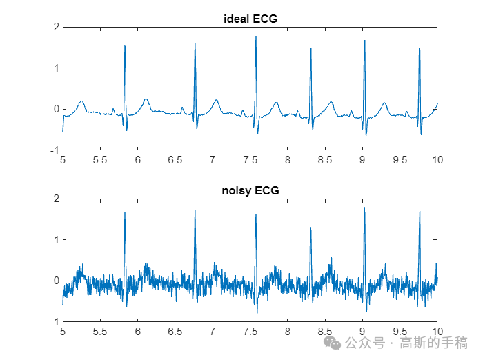
Scaler Kalman filter
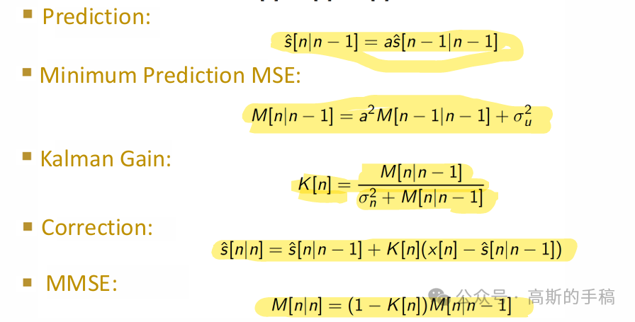
% Initialize the Kalman filter parametersA = 1; % State transition matrixH = 1; % Observation matrixR = 1e-3; % Process noise covariance (adjust as needed)Q = 0.027; % Measurement noise covariance (adjust as needed)x_est = 0; % Initial state estimateP = 1; % Initial estimate covariance
% Create a vector to store the filtered signalfilteredECG = zeros(length(nECG), 1);
% Apply the Kalman filterfor k = 1:length(nECG)    % Prediction step    x_pred = A * x_est;    P_pred = A * P * A' + R;        % Update step    K = P_pred * H' / (H * P_pred * H' + Q); % Kalman gain    x_est = x_pred + K * (nECG(k) - H * x_pred);    P = (1 - K * H) * P_pred;        % Store the filtered estimate    filteredECG(k) = x_est;end
% Plot resultsfigure('Name','Filtered-Kalman filter');subplot(2, 1, 1);plot(t,nECG);title('Noisy ECG Signal');xlabel('Samples');ylabel('Amplitude');xlim([5,10]);
subplot(2, 1, 2);plot(t,filteredECG);title('Filtered ECG Signal (Kalman Filter)');xlabel('Samples');ylabel('Amplitude');xlim([5 10]);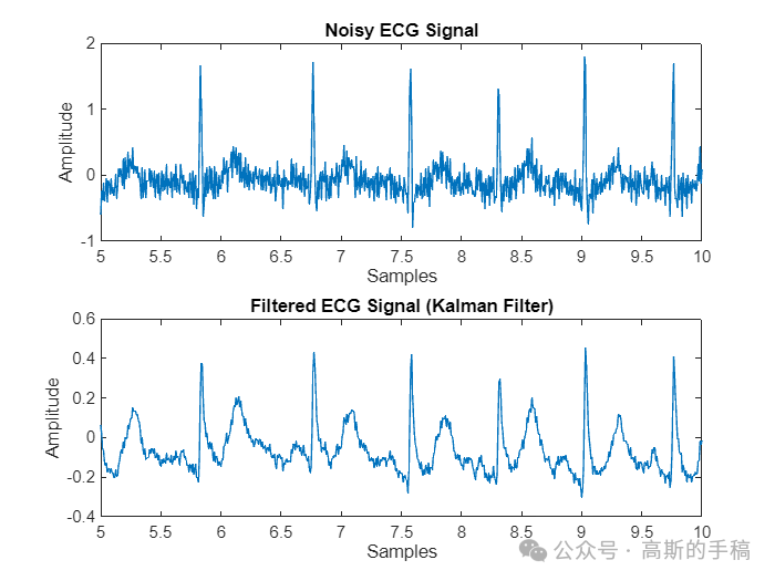
% Initialize the Kalman filter parametersA = 1; % State transition matrixH = 1; % Observation matrixR = 1; % Process noise covariance (adjust as needed)Q = 0.027; % Measurement noise covariance (adjust as needed)x_est = 0; % Initial state estimateP = 1; % Initial estimate covariance
% Create a vector to store the filtered signalfilteredECG = zeros(length(nECG), 1);
% Apply the Kalman filterfor k = 1:length(nECG)    % Prediction step    x_pred = A * x_est;    P_pred = A * P * A' + R;        % Update step    K = P_pred * H' / (H * P_pred * H' + Q); % Kalman gain    x_est = x_pred + K * (nECG(k) - H * x_pred);    P = (1 - K * H) * P_pred;        % Store the filtered estimate    filteredECG(k) = x_est;end
% Plot resultsfigure('Name','Filtered-Kalman filter');subplot(2, 1, 1);plot(t,nECG);title('Noisy ECG Signal');xlabel('Samples');ylabel('Amplitude');xlim([5,10]);
subplot(2, 1, 2);plot(t,filteredECG);title('Filtered ECG Signal (Kalman Filter)');xlabel('Samples');ylabel('Amplitude');xlim([5 10]);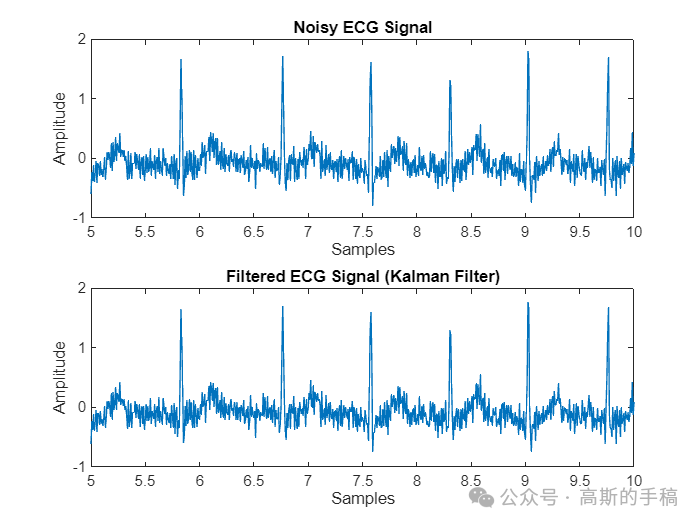
% Initialize the Kalman filter parametersA = 1; % State transition matrixH = 1; % Observation matrixR = 1e-6; % Process noise covariance (adjust as needed)Q = 0.027; % Measurement noise covariance (adjust as needed)x_est = 0; % Initial state estimateP = 1; % Initial estimate covariance
R_array = linspace(1e-3,1,1000);MSE = zeros(size(R_array));
for i = (1:length(R_array))% Create a vector to store the filtered signalfilteredECG = zeros(length(nECG), 1);
% Apply the Kalman filterfor k = 1:length(nECG)    % Prediction step    x_pred = A * x_est;    P_pred = A * P * A' + R_array(i);        % Update step    K = P_pred * H' / (H * P_pred * H' + Q); % Kalman gain    x_est = x_pred + K * (nECG(k) - H * x_pred);    P = (1 - K * H) * P_pred;        % Store the filtered estimate    filteredECG(k) = x_est;endMSE(i) = mean((filteredECG'-idealECG).^2);end
[M, I] = min(MSE)
% Initialize the Kalman filter parametersA = 1; % State transition matrixH = 1; % Observation matrixR = R_array(I); % Process noise covariance (adjust as needed)Q = 0.027; % Measurement noise covariance (adjust as needed)x_est = 0; % Initial state estimateP = 1; % Initial estimate covariance
% Create a vector to store the filtered signalfilteredECG = zeros(length(nECG), 1);
% Apply the Kalman filterfor k = 1:length(nECG) % Prediction step x_pred = A * x_est; P_pred = A * P * A' + R; % Update step K = P_pred * H' / (H * P_pred * H' + Q); % Kalman gain x_est = x_pred + K * (nECG(k) - H * x_pred); P = (1 - K * H) * P_pred; % Store the filtered estimate filteredECG(k) = x_est;end
% Plot resultsfigure('Name','Filtered-Kalman filter');subplot(2, 1, 1);plot(t,nECG);title('Noisy ECG Signal');xlabel('Samples');ylabel('Amplitude');xlim([5,10]);
subplot(2, 1, 2);plot(t,filteredECG);title('Filtered ECG Signal (Kalman Filter)');xlabel('Samples');ylabel('Amplitude');xlim([5 10]);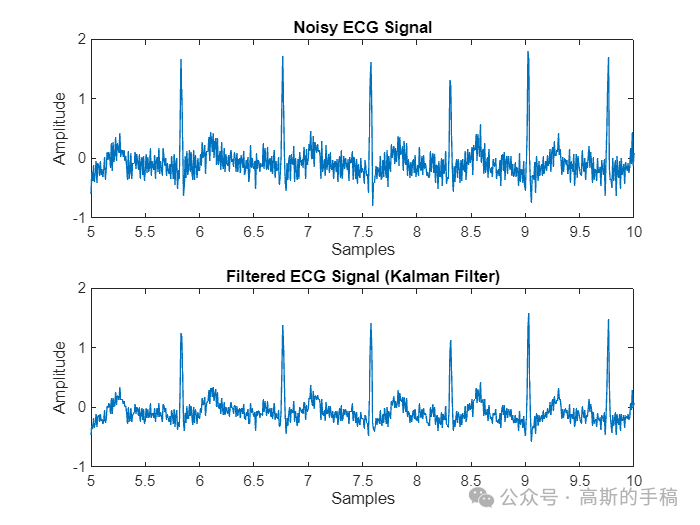
% PSD analysis [p_ideal, f] = periodogram(idealECG, [], [], fs);[p_x, ~] = periodogram(nECG, [], [], fs);[p_filtered, ~] = periodogram(filteredECG, [], [], fs);
figure(6);clf;hold on;plot(f,10*log10(p_ideal));plot(f,10*log10(p_x));plot(f,10*log10(p_filtered));hold off;xlabel('frequency [Hz]');ylabel('power [dB]');title('Power Spectrum Densities')legend ('Ideal ECG','Input signal','filtered signal');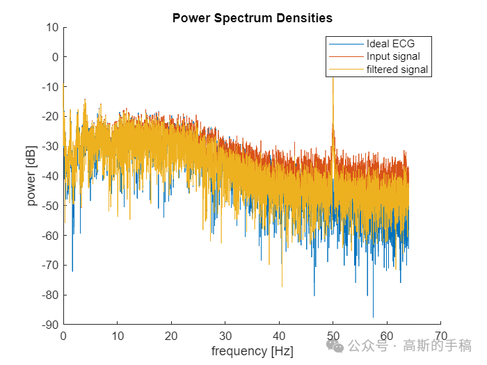
知乎学术咨询:
https://www.zhihu.com/consult/people/792359672131756032?isMe=1
担任《Mechanical System and Signal Processing》《中国电机工程学报》等期刊审稿专家,擅长领域:信号滤波/降噪,机器学习/深度学习,时间序列预分析/预测,设备故障诊断/缺陷检测/异常检测。


分割线分割线分割线分割线分割线分割线分割线分割线分割线分割线


一维神经网络的特征可视化分析-以心电信号为例(Python,Jupyter Notebook)
包括Occlusion sensitivity方法,Saliency map方法,Grad-CAM方法


完整代码可通过知乎付费咨询获得:
https://www.zhihu.com/consult/people/792359672131756032