Understanding MATLAB Robotics Modeling and Simulation Control (5)

Introduction: Continuing the series of Understanding, in the previous article《Understanding | MATLAB Robotics Modeling and Simulation Control (4)》 I believe everyone is quite familiar with the GUI control operations and the data transfer with Simulink. This article mainly addresses the issues left from last time. It mainly includes:

(1) Explanation of other GUI controls. This includes run time, toolbox robot display, and end pose calculation display, using the toolbox inverse kinematics function ikine for end operations.

(2) Adjustment of PID parameters.

1. Explanation of Other GUI Controls

1) The GUI displays the run time, which requires a static text and an editable text field.

a. Drag a static text into the guide interface for run time identification, and make simple settings as follows. Since static text is only used as an identifier, there is no need to write a callback function for it.

Understanding MATLAB Robotics Modeling and Simulation Control (5)

b. Drag an editable text into the guide interface for current run time, and make simple settings as follows.

Note that the tag here is customized as Time, which facilitates the operation of the handle object later. Since the run time starts displaying when the GUI runs, code needs to be written in the automatically generated OpeningFcn of the GUI for time triggering; and a function disptime needs to be written for time display, as follows:

OpeningFcn function:

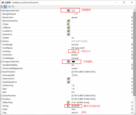
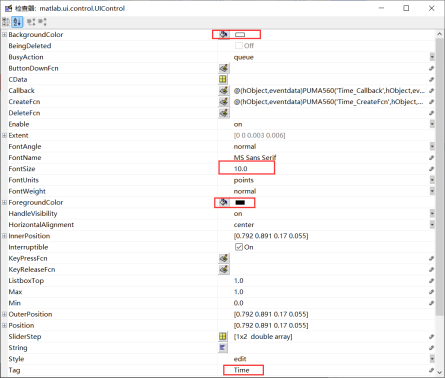
function PUMA560_OpeningFcn(hObject, eventdata, handles, varargin)
clchandles.output = hObject;
%% Run Time
h=timer;   % Timer
handles.T=h;   % Place the timer in the global variable
%set(handles.T,'ExecutionMode','singleShot');  % The timer executes only once, set once.
set(handles.T,'ExecutionMode','fixedRate');   % Timer, executes in a loop, cyclic timing.
set(handles.T,'Period',1);    % Timer, set time interval 1 second
set(handles.T,'TimerFcn',{@disptime,handles});  % Timer triggers the TimerFcn function
% Timer function (TimerFcn) triggers the user-defined function (disptime function)
start(handles.T);   % Start the timer
%% Run immediately display toolbox robot model
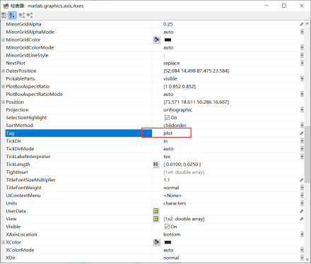
axes(handles.plot)% Specify display area
mdl_puma560   % Import robot model
assignin('base','Robot',p560);% Assign p560 to Robot variable in the base workspace
Robot= evalin('base','Robot');% Specify the variable from the base workspace to the GUI for data sharing
view(3)      % 3D view
Robot.plot([0 0 0 0 0 0]);% Display robot configuration as [0 0 0 0 0 0]
guidata(hObject, handles);

disptime function:

function disptime(hObject, eventdata, handles)
% Custom function to change the content of the edit control to the current time.
set(handles.Time,'String',datestr(now));   % Change the content of the edit control to the current time.

2) GUI displays the robot toolbox model

The robot is displayed in the coordinate area control. Adjust the control size to an appropriate size, double-click to modify and open the property inspector, here only modify the tag to plot (name is self-defined, it is best to have a meaningful name for ease of operation).

Since the robot model is displayed in the coordinate area as soon as the GUI runs, the initial display code is also written in the OpeningFcn function, which can be found in section 1). Corresponding code:<span>axes(handles.plot)% Specify display area<span>。</span></span>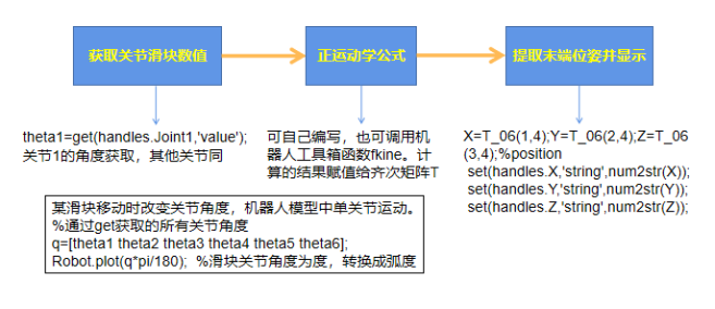

3) End pose calculation display

Requires controls similar to run time controls, static text and editable text, with static text used for identification and editable text for displaying calculation results, the process is roughly as follows.

For example, the code for the robot’s single joint movement and end pose calculation display after moving the joint 1 slider is as follows【Others are similar】:

function Joint1_Callback(hObject, eventdata, handles)
ModelName = 'TestPuma560';% Get the angle
theta1=get(handles.Joint1,'value');
set(handles.edit1,'string',num2str(theta1));  set_param([ModelName '/Slider Gain'],'Gain',num2str(theta1));
theta2=get(handles.Joint2,'value');set(handles.edit2,'string',num2str(theta2));
theta3=get(handles.Joint3,'value');set(handles.edit3,'string',num2str(theta3));
theta4=get(handles.Joint4,'value');set(handles.edit4,'string',num2str(theta4));
theta5=get(handles.Joint5,'value');set(handles.edit5,'string',num2str(theta5));
theta6=get(handles.Joint6,'value');set(handles.edit6,'string',num2str(theta6));% Data transmission to Simulink
set_param([ModelName '/Slider Gain1'],'Gain',num2str(theta2));
set_param([ModelName '/Slider Gain2'],'Gain',num2str(theta3));
set_param([ModelName '/Slider Gain3'],'Gain',num2str(theta4));
set_param([ModelName '/Slider Gain5'],'Gain',num2str(theta5));
set_param([ModelName '/Slider Gain6'],'Gain',num2str(theta6));% Forward kinematics calculation
rpy=zeros(1,3);        a2 = 0.4318;        a3 = 0.0203;        d3 = 0.1501;        d4 = 0.4318;
t1=theta1;t2=theta2; t3=theta3; t4=theta4; t5=theta5; t6=theta6;             T_01 = tmat(0, 0, 0, t1);
        T_12 = tmat(90, 0, 0, t2);
        T_23 = tmat(0, a2, d3, t3);
        T_34 = tmat(-90, a3, d4, t4);
        T_45 = tmat(90, 0, 0, t5);
        T_56 = tmat(-90, 0, 0, t6); % Each link frame to base frame transformation        T_02 = T_01*T_12;
        T_03 = T_02*T_23;
        T_04 = T_03*T_34;
        T_05 = T_04*T_45;
        T_06 = T_05*T_56;
     X=T_06(1,4);Y=T_06(2,4);Z=T_06(3,4);%position
R=T_06;if abs(abs(R(1,3)) - 1) < eps  % when |R13| == 1        % singularity
rpy(1) = 0;  % roll is zero
if R(1,3) > 0
rpy(3) = atan2( R(3,2), R(2,2));   % R+Y        
else
rpy(3) = -atan2( R(2,1), R(3,1));   % R-Y        
end
rpy(2) = asin(R(1,3));
else        rpy(1) = -atan2(R(1,2), R(1,1));
        rpy(3) = -atan2(R(2,3), R(3,3));
        rpy(2) = atan(R(1,3)*cos(rpy(1))/R(1,1));    end
RPY=rpy*180/pi;
Rall=round(RPY(1));Pitch=round(RPY(2));Yaw=round(RPY(3));
set(handles.X,'string',num2str(X));
set(handles.Y,'string',num2str(Y));
set(handles.Z,'string',num2str(Z));
set(handles.R,'string',num2str(Rall));
set(handles.P,'string',num2str(Pitch));
set(handles.Yr,'string',num2str(Yaw));
q=[theta1 theta2 theta3 theta4 theta5 theta6];  Robot= evalin('base','Robot');  handles.plot;Robot.plot(q*pi/180);%   Robot.plot3d(q*pi/180, 'view',[-138 8]);  T=Robot.fkine(q*pi/180);hold on
plot3(T.t(1,1),T.t(2,1),T.t(3,1),'.','LineWidth',3,'color','r');

The forward kinematics calculation for the end pose calls the tmat function:

function T = tmat(alpha, a, d, theta)% Improved DH method, coordinate transformation process as seen in Craig
alpha = alpha*pi/180;    %Note: alpha is in radians.
theta = theta*pi/180;    %Note: theta is in radians.
c = cos(theta);s = sin(theta);ca = cos(alpha);sa = sin(alpha);
T = [c -s 0 a; s*ca c*ca -sa -sa*d; s*sa c*sa ca ca*d; 0 0 0 1];

4) Using the toolbox inverse kinematics function ikine for Cartesian space operations at the end

The controls selected here are static text and a button. The static text still serves only as an identifier, and the button is pressed as the input for the end position vector, using inverse kinematics to obtain the joint angles, which are then passed to the robot.

The callback function for the button is basically the same, below is the code for changing the robot’s end X:

X-button callback code:

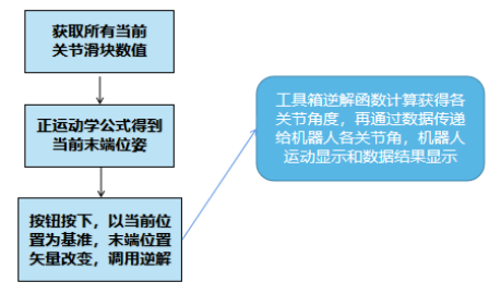
function pushbutton3_Callback(hObject, eventdata, handles)
Robot= evalin('base','Robot');
theta1=get(handles.Joint1,'value');
theta2=get(handles.Joint2,'value');
theta3=get(handles.Joint3,'value');
theta4=get(handles.Joint4,'value');
theta5=get(handles.Joint5,'value');
theta6=get(handles.Joint6,'value');
q0=[theta1 theta2 theta3 theta4 theta5 theta6];
T0=Robot.fkine(q0*pi/180);
R=[T0.n T0.o  T0.a];% Directly call the forward kinematics function
numMats = size(R,3);
H = zeros(4,4,numMats,'like',R);
H(1:3,1:3,:) = R;
H(4,4,:) = ones(1,1,numMats,'like',R);
H(1:3,4)=T0.t;% SE3 xyzMovement To Homogeneous matrix
Hinit=H;
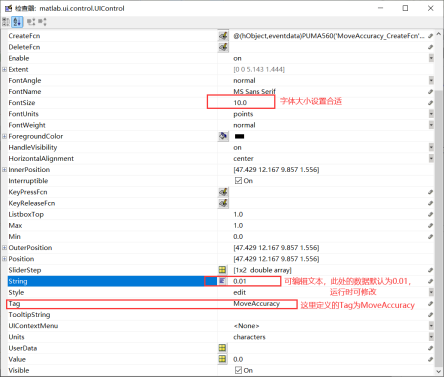
offset=str2double(get(handles.MoveAccuracy,'string'));% Movement step length, precision
H(1:1 ,4:4)=Hinit(13)+offset;% Take the current end as a reference for end movement
%Hinit(13) is the number in the 13th position of the matrix, which is the X coordinate in the homogeneous matrix.
Hmove=H;
Q=Robot.ikine(Hmove);% Call the inverse kinematics function to obtain joint values
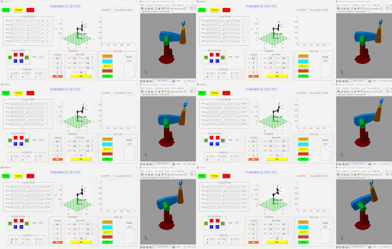
handles.plot;Robot.plot(Q);% Display end movement
theta1=Q(1)*180/pi;
theta2=Q(2)*180/pi;
theta3=Q(3)*180/pi;
theta4=Q(4)*180/pi;
theta5=Q(5)*180/pi;
theta6=Q(6)*180/pi;
% Set slider movement and corresponding angle display
set(handles.Joint1,'value',theta1);
set(handles.Joint2,'value',theta2);
set(handles.Joint3,'value',theta3);
set(handles.Joint4,'value',theta4);
set(handles.Joint5,'value',theta5);
set(handles.Joint6,'value',theta6);
set(handles.edit1,'string',num2str(theta1));
set(handles.edit2,'string',num2str(theta2));
set(handles.edit3,'string',num2str(theta3));
set(handles.edit4,'string',num2str(theta4));
set(handles.edit5,'string',num2str(theta5));
set(handles.edit6,'string',num2str(theta6));
% Operation for Simulink
ModelName = 'TestPuma560';
set_param([ModelName '/Slider Gain'],'Gain',num2str(theta1));
set_param([ModelName '/Slider Gain1'],'Gain',num2str(theta2));
set_param([ModelName '/Slider Gain2'],'Gain',num2str(theta3));
set_param([ModelName '/Slider Gain3'],'Gain',num2str(theta4));
set_param([ModelName '/Slider Gain5'],'Gain',num2str(theta5));
set_param([ModelName '/Slider Gain6'],'Gain',num2str(theta6));
% Display end movement trajectory, X is red  
T=Robot.fkine(Q);
hold on
plot3(T.t(1,1),T.t(2,1),T.t(3,1),'.','LineWidth',3,'color','r');
X=T.t(1,1);
Y=T.t(2,1);
Z=T.t(3,1);
set(handles.X,'string',num2str(X));
set(handles.Y,'string',num2str(Y));
set(handles.Z,'string',num2str(Z));

The control of inverse kinematics in the GUI sets the step length of the end position vector change, using a static text as an identifier. The static text can be dragged in and renamed. The editable text can modify data at runtime and be obtained in the position button callback.

The line in the above code:

offset=str2double(get(handles.MoveAccuracy,’string’));

The editable text is modified as follows:

Effect: (Here only the position vector is controlled, if the posture needs to be controlled, controls can be added in the same way.)

2. Adjustment of PID Parameters

Double-click to open the PID controller, the default parameters are as follows.

In this case, replace the angle input for joint 1 with a sine wave module for testing.

Using the Scope oscilloscope, the angle tracking situation is as follows, and there is obviously an error:

Therefore, adjust the PID parameters. Here, use the PID automatic parameter tuning tool. Run the model once, then double-click the PID control module and click the Tune button.

Adjust the response time and robustness (overshoot), the solid line will automatically update the adjusted response.

After obtaining a satisfactory response, we choose update to update the PID parameters to Simulink.

After the PID parameters are automatically generated, click apply.

Now run the model. You can see that the angle tracking situation of joint 1 has improved a lot, the error is very small, indicating that the adjustment of the PID parameters for joint 1 is complete, and other joints can be adjusted in a similar manner.

So far, we have basically solved the problems left in Understanding 4.

Postscript: The author has limited ability, if there are any errors, please point them out in time.

(1) For PID parameter adjustment related references, please refer to:

https://zhuanlan.zhihu.com/p/74131690

https://zhuanlan.zhihu.com/p/139945063

Book: “Advanced PID Control MATLAB Simulation” by Liu Jinkun

(2) For learning GUI design without guide, please refer to:

https://www.bilibili.com/video/BV1mK411p7c3

(3) Reference books for GUI design:“Introduction and Practice of MATLAB GUI Design”

(4) For learning the Robotics Toolbox, please refer to:

https://www.bilibili.com/video/BV1MK4y1k7je

———The above

Benefits

Please reply “Member Exchange” in the background of the GuYueJu public account for those who participated in the GuYueJu discount event last week to receive 3 months of GuYue Academy membership.

Related posts

Leave a Comment Cancel reply