When it comes to diagnostic trials, they are widely applied: to evaluate whether the results of two methods or instruments are consistent, we need diagnostic trials; to see if two doctors diagnose the same group of patients consistently, diagnostic trials are necessary; to assess the consistency of diagnostic results for the same group of patients on two occasions, diagnostic trials are also required, and so on…
In short, the focus of diagnostic trials is on “consistency”, meaning that observations using two instruments (methods/evaluators) or at two different times should yield consistent results within an acceptable error range.There are many methods to evaluate the degree of consistency, such as Kappa value, Kendall’s coefficient of concordance, intraclass correlation coefficient (ICC), etc. However, choosing the right method is not easy, so let’s clarify this together!
Paired χ2 Test vs. Consistency Test
The paired χ2 test (McNemar test) and Kappa consistency test can both be used forthe analysis of paired contingency tables (Table 1), for example, to compare the diagnostic value of ultrasound and CT scan for acute appendicitis, but each has its own focus.
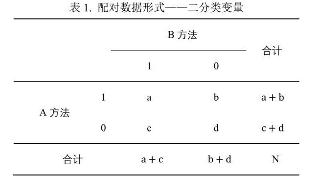
(1) The calculation methods of the two are different
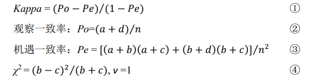
As can be seen from ①②③, the Kappa calculation process utilizes all data in the four-cell table (a, b, c, d), while formula ④ indicates that the paired χ2 test only uses the “inconsistent” data (b and c) from the four-cell table.
(2) The information provided by the two is different
Consistency tests can not only clarify whether there is consistency between two methods but also calculate the Kappa value, thereby evaluating the degree of consistency. It is currently believed that Kappa<0 indicates very poor consistency (which is unlikely to occur in practice); 0-0.20 indicates weak; 0.21-0.40 indicates moderate; 0.41-0.60 indicates moderate; 0.61-0.80 indicates high; and 0.81-1.00 indicates very strong.
The paired χ2 test can only indicate whether the difference in the positive (or negative) detection rates of the two methods is statistically significant, but it obscures a problem, namely, it does not distinguish between true positives (true negatives) and false positives (false negatives) for the positive (or negative) detection rates of the two methods. In fact, we are more interested in how consistently both methods detect true patients or non-patients,which highlights the importance of Kappa.
For detailed operations, click the link below: SPSS detailed operations: consistency test and paired chi-square test / SPSS operations: consistency test, how to calculate Kappa value?
Weighted Kappa and Kendall’s Tb Coefficient
In addition to the unordered categorical variables mentioned above, we also encounter someordered categorical data (ordinal data) results (Table 2), such as laboratory results of “-, ±, +, ++, +++”, which require the use of weighted Kappa coefficient and Kendall’s Tb coefficient to evaluate the consistency of diagnostic trials.
The weighted Kappa coefficient is a generalization of the simple Kappa coefficient, which quantifies the two evaluation results using a weighted method. Earlier, an article introducing weighted Kappa was published: SPSS operations: consistency test for ordered categorical variables—weighted Kappa, if you are not familiar, you can review it again.
Here, let’s focus onKendall’s Tb coefficient[1], which is a non-parametric method that can be used toevaluate the consistency of two groups of ordered categorical data.
The basic principle is to rank the two sets of measurements and convert them into ranks, checking whether the order of the two sets of values is consistent. If the orders of the two sets are completely the same, then Tb=1; if the orders are completely opposite, then Tb=-1. Let’s use the example of “weighted Kappa SPSS operations” to introduce how to implement Kendall’s Tb coefficient.
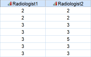
A certain hospital intends to analyze the consistency of different radiologists’ diagnoses of disease severity. Two radiologists (Radiologist 1 and Radiologist 2) are recruited to assess the MRI results of 50 subjects and provide clinical diagnoses rated from Grade I (mildest) to Grade V (most severe) (in the database, Grade I to Grade V are assigned values of 1 to 5). Some data is as follows:
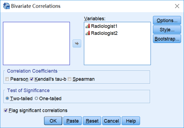
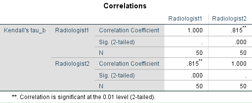
In SPSS, select Analyze → Correlate → Bivariate → display the “Bivariate Correlations” main dialog box (as shown below) → place “Radiologist 1 and Radiologist 2” in the “Variables” box → select “Kendall’s tau-b” → OK
The results show, Kendall’s Tb coefficient = 0.815 (P<0.001), which is close to the weighted Kappa coefficient (0.803, P<0.001), both indicating that the two radiologists have a high consistency in diagnosing the severity of disease in 50 subjects.
Paired t-test/Correlation Analysis
vs.
Intraclass Correlation Coefficient (ICC)
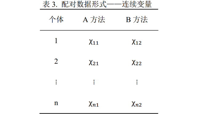
Having discussed the consistency test for categorical variables, what should we do whenwe encounter continuous variables (Table 3)? Most people immediately resort to correlation analysis and paired t-tests, but in fact, neither of these methods can determine “whether there is consistency”. Why? Let me explain slowly.
(1) Correlation Analysis
Assuming the results obtained by the two methods are viewed as two variables, correlation analysis can determine whether there is a correlation between the variables (for those still confused, click: SPSS super detailed tutorial: Pearson correlation analysis), but it cannot determine whether they have consistency. Why? Let’s illustrate with some data from the tutorial on “SPSS operations: Intraclass Correlation Coefficient (ICC)”.
Now assume there are 2 researchers measuring the blood glucose levels of 10 subjects using the same diagnostic trial.
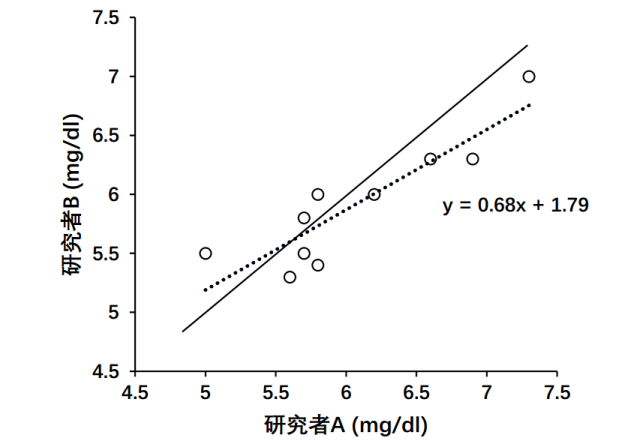
Figure 1. Blood glucose levels measured by two researchers
First, look at the scatter plot (the magic tool for correlation analysis, highly recommended!), using the blood glucose levels measured by researcher A and B as the two coordinates, plotting the paired data on a Cartesian plane (Figure 1).
Consistency testing means analyzing the error of all data to the line Y=X (the solid line in Figure 1), while correlation (bivariate correlation analysis and simple linear regression are equivalent) means analyzing the residuals to the line Y=aX+b (usually a≠1, b≠0) (the dashed line in Figure 1).
Furthermore, correlation analysis is easily affected by outliers. As shown in Figure 1, the correlation between the blood glucose levels measured by the two researchers is quite good (r=0.89), but if we remove the point in the upper right corner, the correlation coefficient would drop to r=0.81. Clearly, using the correlation coefficient to measure the relationship between the blood glucose levels of the two researchers is inappropriate.
Therefore, correlation analysis cannot replace consistency testing.
(2) Paired t-test
The paired t-test is suitable for paired data, and its principle is to treat the difference d between the results of the two methods as a variable, with the prerequisite that this variable follows a normal distribution with unknown variance, aiming to examine whether there is a significant difference in the average of the two methods (see: paired sample t-test, the most complete SPSS operation tutorial).
H0: μd=0, there is no difference in the means of the two populations;
H1: μd≠0, there is a difference in the means of the two populations.
If P>0.05, it only indicates that the current evidence is insufficient to conclude that the average difference between the two methods is not equal to 0, and does not adequately reflect the consistency between the two. In fact, keeping the mean and standard deviation of the difference unchanged, when the sample size is large enough, a result of P<0.05 will always be obtained. Clearly, it is inappropriate to use the paired t-test to assess the quality of consistency in diagnostic trials.
(3) Intraclass Correlation Coefficient (ICC)
The intraclass correlation coefficient (ICC)[2,3] can be used to evaluate the consistency or reliability of different measurement methods or evaluators on the same quantitative measurement results.

The larger the ICC, the smaller the variation caused by systematic errors and random errors. The ICC value ranges from 0 to 1, generally considered: ICC>0.75 indicates good consistency, 0.40~0.75 is average, and <0.40 is poor.
Data simulation analysis has found[3] that the paired t-test is sensitive to systematic errors (different measurement methods, instruments, evaluators), but cannot simultaneously account for random errors (variability of the subjects themselves), while the simple correlation coefficient is just the opposite. Therefore, the paired t-test and simple correlation analysis are evidently one-sided, unable to simultaneously consider random and systematic errors, and conclusions drawn from them regarding consistency may be incorrect.
Although the calculation model of the intraclass correlation coefficient is still debated, it considers the influence of both systematic and random errors and is not affected by data type, thus having a significant advantage over paired t-tests and simple correlation analyses.
For how to calculate ICC, you can click the link below:SPSS operations: Intraclass Correlation Coefficient (ICC)
References
1. Rank Correlation Methods, 4th Edition. 1970.
2. Chinese Health Statistics. 2011; 28:497-500.
3. Chinese Health Statistics. 2011; 28:40-2.

Click the bottom left corner “Read the original text” to learn over 70 free SPSS tutorials, over 30 R tutorials, and more free research tutorials!