Previously, the derivation of the least squares method was introduced, which is widely used in function differentiation. When using it, existing tools can be directly utilized to solve (for example, using A\b in MATLAB to solve for x). However, sometimes it is necessary to handle constraint problems, so it is essential to master the constrained least squares method for solving and its application.
Problem Description
The constrained least squares problem can be expressed as:
Where:
- is the design matrix
- is the observation vector
- is the constraint matrix
- is the constraint value vector
- is the parameter vector to be solved
Derivation Using the Lagrange Function Method
1. Construct the Lagrange Function
Introduce the Lagrange multiplier vector , and construct the Lagrange function:
Expanding gives:
2. Calculate the Partial Derivative
Take the partial derivative with respect to :
Set the partial derivative to zero:
Rearranging gives:
Take the partial derivative with respect to :
Set the partial derivative to zero (i.e., the constraint condition):
3. Construct the KKT System
Combine equations (1) and (2) into the KKT system:
This is a linear system, and the optimal solution and the corresponding Lagrange multipliers can be obtained by solving this equation set.
❝
Note: The KKT conditions transform the original problem from “a constrained minimization problem” to “a problem of solving a system of equations”, which is the KKT system.
4. Form of the Solution
If is invertible, an analytical solution can be obtained. From equation (1), we have:
Substituting into equation (2):
Rearranging gives:
Solving for :
Then substituting back to find :
Application: Constrained Cubic Polynomial Fitting
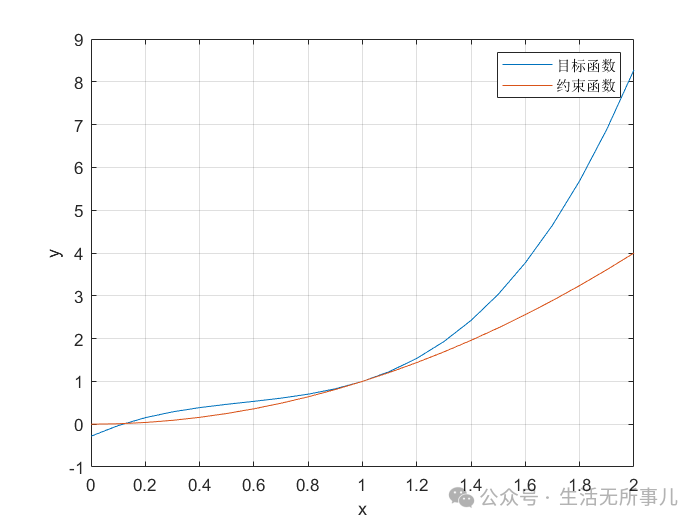
Applying constrained least squares to fit a cubic polynomial (objective function):
Where the objective function is required to be tangent at (1, 1) and , thus the constraint condition is transformed into:
MATLAB Code Implementation
clc;
clear;
close all;

x= 0:0.1:2;
x=x';
y=x.^3;

x0=1;
y0=x0^3;
dy0 = 2*x0;

n = length(x);
A = [x.^3 x.^2 x ones(n, 1)];

C = [x0^3 x0^2 x0 1;
    3*x0^2 2*x0 0];
d = [y0; dy0];

M=[A'*A C';
    C zeros(2, 2)];
B=[A'*y; d];

p = M\B;

dy1 = 3*p(1)*x0.^2 + 2*p(2)*x0 + p(3);
figure
y1 = p(1)*x.^3 + p(2)*x.^2 + p(3)*x + p(4);
y2 = x.^2;
plot(x, y1)
hold on
plot(x, y2)
grid on
xlabel('x')
ylabel('y')
legend('Objective Function', 'Constraint Function')
The fitting result is as follows:
-END-If you find this article helpful, feel free to like and follow!!!